Eilmer Reference Manual, v5
Eilmer is a multi-physics analysis code with an emphasis on the simulation of compressible gas flows. In broad terms, the workflow for a simulation consists of 3 steps:
-
pre-processing;
-
running a simulation; and
-
post-processing.
A simulation is set up by writing input scripts (possibly separately for
grid and flow definition) and running them through the pre-processors,
such as prep-grid and prep-sim.
The lmr run command is used to launch a simulation for single node jobs,
and there are MPI-flavoured executables for launching distributed-memory
parallel jobs, for example, on cluster computers.
There are a variety of post-processing tools to support extraction and
visualisation of the simulated flow field data.
Commonly users will call the snapshot2vtk command to produce
VTK files for viewing in a tool such as Paraview.
The following sections provide brief details on many items that
might go into your input script.
Note that this document is for reference, after you have read the guides at
https://gdtk.uqcloud.net/docs/eilmer/user-guide/ .
1. Configuration options
There are a large number of configuration options that can be set in the input script. The options are set in the input script by adding lines of the form:
config.option = value
Here are all of the available configuration options and the default values if left unset. Note you do not have to set all of these values in the input script. In a typical input script, one might set 10-15 input variables.
1.1. Solver mode
config.solver_mode-
string, default:
'transient'
The options are:'transient'or'steady'
1.2. Geometry
config.dimensions-
int, default:
2
Spatial dimensionality, 2 or 3 config.axisymmetric-
bool, default:
false
Sets axisymmetric mode for 2D geometries. The axis of rotation aligns with the x-axis (at y=0).
1.3. Time-stepping
config.gasdynamic_update_scheme-
string, default:
'predictor-corrector'
The options are:'euler','pc','predictor-corrector','midpoint','classic-rk3','tvd-rk3','denman-rk3','moving-grid-1-stage','moving-grid-2-stage','backward_euler','implicit_rk1'. Most of the update schemes are explicit, except for the last two listed here. Note that'pc'is equivalent to'predictor-corrector'. If you want time-accurate solutions, use a two- or three-stage explicit stepping scheme, otherwise, (explicit) Euler stepping has less computational expense but you may get less accuracy and the code will not be as robust for the same CFL value. For example the shock front in the Sod shock tube example is quite noisy for Euler stepping at CFL=0.85 but is quite neat with any of the two- or three-stage stepping schemes at the same value of CFL. The explicit midpoint and predictor-corrector schemes produce a tidy shock up to CFL = 1.0 and the rk3 schemes still look tidy up to CFL = 1.2. If you care mainly about the end result, you might be able to use an implicit scheme with larger CFL number. We have run the'backward_euler'scheme up to a CFL value of 50 for some of the turbulent flat-plate examples. The implicit schemes are more expensive than the low-order explicit schemes, per time-step and, at large CFL numbers, will not be time accurate. The trade-off will be something that you have to explore but, if you care only about a steady state, the'backward_euler'scheme may get you there more quickly than any of the explicit schemes. Your mileage will vary. Note that you may use dashes or underscores when spelling the scheme names. config.fixed_time_step-
boolean, default:
false
Normally, we allow the time step size to be determined from cell conditions and CFL number. Settingconfig.fixed_time_step=trueforces the time step size to be unchanged fromconfig.dt_init. config.cfl_value-
float, default:
0.5
The CFL number is ratio of the time-step divided by the time for the fastest signal to cross a cell. The time-step adjustment process tries to set the time-step for the overall simulation to a value such that the maximum CFL number for any cell is at thiscfl_value. If you are having trouble with a simulation that has lots of sudden flow field changes, decreasing the size ofcfl_valuemay help. config.cfl_schedule-
table of float pairs, default
{{0.0, config.cfl_value},}
If you want to vary thecfl_valueas the simulation proceeds, possibly starting with small values and then increasing them as the flow field settles to something not too difficult for the flow solver, you can specify a table of{time,cfl_value}pairs that are interpolated by the solver. Outside the specified range of times, thecfl_valuewill be the closest end-point value. config.dt_init-
float, default:
1.0e-3
Although the computation of the time step size is usually automatic, there might be cases where this process does not select a small enough value to get the simulation started stably. For the initial step, the user may override the computed value of time step by assigning a suitably small value toconfig.dt_init. This will then be the initial time step (in seconds) that will be used for the first few steps of the simulation process. Be careful to set a value small enough for the time-stepping to be stable. Since the time stepping is synchronous across all parts of the flow domain, this time step size should be smaller than half of the smallest time for a signal (pressure wave) to cross any cell in the flow domain. If you are sure that your geometric and boundary descriptions are correct but your simulation fails for no clear reason, try setting the initial time step to a very small value. For some simulations of viscous hypersonic flow on fine grids, it is not unusual to require time steps to be as small as a nanosecond. config.dt_max-
float, default:
1.0e-3
Maximum allowable time step (in seconds). Sometimes, especially when strong source terms are at play, the CFL-based time-step determination does not suitably limit the size of the allowable time step. This parameter allows the user to limit the maximum time step directly. config.viscous_signal_factor-
float, default:
1.0
By default, the full viscous effect for the signal calculation will be used within the time-step calculation. It has been suggested that the full viscous effect may not be needed to ensure stable calculations for highly-resolved viscous calculations. A value of0.0will completely suppress the viscous contribution to the signal speed calculation but you may end up with unstable stepping. It’s a matter of try a value and see if you get a larger time-step while retaining a stable simulation. config.stringent_cfl-
boolean, default:
false
The default action for structured grids is to use different cell widths in each index direction. Settingconfig.stringent_cfl=truewill use the smallest cross-cell distance in the time-step size check. config.cfl_count-
int, default:
10
The number of time steps between checks of the size of the time step. This check is expensive so we don’t want to do it too frequently but, then, we have to be careful that the flow does not develop suddenly and the time step become unstable. config.max_time-
float, default:
1.0e-3
The simulation will be terminated on reaching this value of time. config.max_step-
int, default:
100
The simulation will be terminated on reaching this number of time steps. You will almost certainly want to use a larger value, however, a small value is a good way to test the starting process of a simulation, to see that all seems to be in order. config.dt_plot-
float, default:
1.0e-3
The whole flow solution will be written to disk when this amount of simulation time has elapsed, and then again, each occasion the same increment of simulation time has elapsed. config.dt_history-
float, default:
1.0e-3
The history-point data will be written to disk repeatedly, each time this increment of simulation time has elapsed. To obtain history data, you will also need to specify one or more history points. config.with_local_time_stepping-
boolean, default:
false
If a steady-state solution is sought, then it is possible to accelerate the explicit time-stepping scheme by allowing each cell in the domain to integrate in time with their own time-step that satisfies only the local CFL condition. This is sometimes referred to as Local Time-Stepping (LTS). Settingconfig.with_local_time_stepping=trueenables this mode of time-stepping. Note that this mode of time-stepping is only suitable for steady-state simulations. config.local_time_stepping_limit_factor-
int, default:
10000
To improve the stability of simulations that enableconfig.with_local_time_stepping, users can limit the largest allowable local time-step as a function of the smallest global time-step. The allowable time-step for each cell is set to be the minimum of the cell’s local time-step and the global minimum time-step multiplied byconfig.local_time_stepping_limit_factor. Theconfig.local_time_stepping_limit_factoris typically set to a value between 500 and 10000. config.residual_smoothing-
boolean, default:
false
Residual smoothing essentially applies an averaging filter on the residuals during the time-integration procedure. Residual smoothing has two advantages: (1) The averaging increases the allowable CFL for a particular explicit time-stepping scheme; and (2) The averaging ensures that the local time-step for two adjacent cells doesn’t differ by a large magnitude when usingconfig.with_local_time_stepping, this has a stabilising effect. config.residual_smoothing_type-
string, default:
'explicit'
The options are:'explicit','implicit'. Whenconfig.residual_smoothing=true, the residuals can either be smoothed via an explicit averaging method or an implicit averaging method. Explicit averaging has less computational expense, however, implicit averaging typically results in a larger stable time step. config.residual_smoothing_weight-
float, default:
0.2
A weighting factor used in the residual averaging whenconfig.residual_smoothing=true. config.residual_smoothing_iterations-
int, default:
2
The number of Jacobi iterations used for the implicit residual averaging whenconfig.residual_smoothing=trueandconfig.residual_smoothing_type='implicit'.
1.4. Block marching
config.block_marching-
boolean, default:
false
Normal time iteration proceeds on all blocks simultaneously, however, such a time-marching calulation may be very expensive computationally. Settingconfig.block_marching=trueenables a sequencing of the time integration such that at any one instant, only two slices of blocks are being integrated. The i-direction is the marching direction and the assumed dominant (supersonic) flow direction. The blocks are assumed to be in a regular array with a fixed number of blocks in the j- and k-directions to the entire flow domain. config.nib,config.njb,config.nkb-
int default:
1,1,1
are the number of blocks in each index direction. To make the best of block marching, you should haveconfig.nibset to a fairly large number. Since the array of blocks is assumed regular, you cannot have very complicated geometries. Simple ducts, nozzles and plates are the intended applications. As seen in the examples, it may be convenient to define the full domain with one or more calls to the constructorFBArray:new. There is a restriction that the overall flow domain be assembled as a single structured array ofFlowBlockobjects. config.propagate_inflow_data-
boolean, default:
false
By default, the integration begins in each set of blocks from the initial gas state set up in the preparation phase of the simulation. Some advantage may be gained following integration of the first block slices by initializing subsequent block slices with the downstream (east boundary) flow states. Settingconfig.propagate_inflow_data=truepropagates these data across each new block slice, before the integration process for the slice begins. config.save_intermediate_results-
boolean, default:
false
Usually, a single set of solution files (after marching over all block slices) is all that is required. Sometimes, when debugging a troublesome calculation, it may be useful to have a solution written after the time-integration process for each pair of block slices. Set this parametertrueto get these intermediate solutions written.
1.5. Spatial reconstruction
config.interpolation_order-
int, default:
2
Before applying the flux calculator, high-order reconstruction is applied. Settingconfig.interpolation_order=1results in no reconstruction of intra-cell flow properties. config.interpolation_delay-
float, default:
0.0
The time (in seconds) to wait before increasing the interpolation order. If the delay is enabled, the simulation will begin usinginterpolation_order=1. After the delay time, the interpolation order will switch to that specified in the configuration. This delay is useful to help with robustness during transient starts because the first order spatial reconstruction is very reliable (albeit less accurate as compared to high order reconstruction). config.apply_limiter-
boolean, default:
true
By default, we apply a limiter to the flow-field reconstruction. config.extrema_clipping-
boolean, default:
true
By default, we do extrema clipping at end of each scalar-field reconstruction. Settingconfig.extrema_clipping=falsesuppresses clipping. config.thermo_interpolator-
string, default:
'rhou'
String to choose the set of interpolation variables to use in the interpolation, options are'rhou','rhop','rhoT'and'pT'.
1.6. Flux calculator
config.flux_calculator-
string, default:
'adaptive_hanel_ausmdv'
Selects the flavour of the flux calculator. Options are:-
'efm'A cheap and very diffusive scheme by Pullin and Macrossan. For most hypersonic flows, it is too diffusive to be used for the whole flow field but it does work very nicely in conjunction with AUSMDV, especially for example, in the shock layer of a blunt-body flow. -
'ausmdv'A good all-round scheme with low-diffusion for supersonic flows. -
'adaptive_efm_ausmdv'A blend of the low-dissipation AUSMDV scheme for the regions away from shocks with the much more diffusive EFM used for cell interfaces near shocks. It seems to work quite reliably for hypersonic flows that are a mix of very strong shocks with mixed regions of subsonic and supersonic flow. The blend is controlled by the parametersconfig.compression_toleranceandconfig.shear_tolerancethat are described below. -
'ausm_plus_up'Implemented from the description by MS Liou (2006). It should be accurate and robust for all speed regimes. It is the flux calculator of choice for very low Mach number flows, where the fluid behaviour approaches the incompressible limit. For best results, you should set the value ofM_inf. -
'hlle'The Harten-Lax-vanLeer-Einfeldt (HLLE) scheme. It is somewhat dissipative and is the only scheme usable with MHD terms. -
'adaptive_hlle_ausmdv'As for'adaptive_efm_ausmdv'but with the dissipative scheme being the HLLE flux calculator. -
'hanel'The Hanel-Schwane-Seider scheme, from their 1987 paper. It also dissipative and is somewhat better behaved than our EFM implementation. -
'adaptive_hanel_ausmdv'As for'adaptive_efm_ausmdv'but with the dissipative scheme being the Hanel-Schwane-Seider flux calculator. -
'roe'The Phil Roe’s classic linearized flux calculator. -
'adaptive_hlle_roe'A blend of Roe’s low-dissipation scheme and the more dissipative HLLE flux calculator. -
'adaptive_ausmdv_asf'A blend of Summation-by-Parts method of Fisher (high order, low-dissipation scheme) and the ausmdv method.
-
The default adaptive scheme is a good all-round scheme that uses AUSMDV away from shocks and Hanel-Schwane-Seider flux calculator near shocks.
Any of the schemes with the prefix 'adaptive' can be used in a blended mode
if the shock_detector_smoothing is enabled.
config.compression_tolerance-
float, default:
-0.30
The value of relative velocity change (normalised by local sound-speed) across a cell-interface that triggers the shock-point detector. A negative value indicates a compression. When an adaptive flux calculator is used and the shock detector is triggered, the more-dissipative flux calculation will be used in place of the default low-dissipation calculation. A value of-0.05seems OK for the Sod shock tube and sharp-cone inviscid flow simulations, however, a higher value is needed for cases with viscous boundary layers, where it is important to not have too much numerical dissipation in the boundary layer region. config.shear_tolerance-
float, default:
0.20
The value of the relative tangential-velocity change (normalised by local sound speed) across a cell-interface that suppresses the use of the high-dissipation flux calculator even if the shock detector indicates that high-dissipation scheme should be used within the adaptive flux calculator. The default value is experimentally set at 0.20 to get smooth shocks in the stagnation region of bluff bodies. A smaller value (say,0.05) may be needed to get strongly expanding flows to behave when regions of shear are also present. config.M_inf-
float, default:
0.01
representative Mach number for the free stream. Used by theausm_plus_upflux calculator.
config.shock_detector_smoothing-
int, default =
0
How many iterations of shock detector averaging. Higher values spread the influence of the shock detector further from the shock, increasing numerical dissipation but providing a smoother transition between flux calculators in adaptive schemes.
|
Tip
|
You can read more about this in the technical note Hybrid fluxes, shock detection and smoothing. |
config.strict_shock_detector-
boolean, default:
true
If this is true then any face that is part of a cell with S>0 will have its own S value set to 1. This is to emulate legacy behaviour and thus defaults to true. For true blending of fluxes this should be set to false. config.frozen_shock_detector-
boolean, default:
false
If set to true, the shock detector field will be frozen after the number of time steps prescribed by config.shock_detector_freeze_step. Used to prevent flickering of adaptive flux methods between their constituent flux calculators. config.shock_detector_freeze_step-
int, default:
1000
The time step at which the shock detector field will be frozen.
1.7. Viscous effects
config.viscous-
boolean, default:
false
If settrue, viscous effects will be included in the simulation. config.separate_update_for_viscous_terms-
boolean, default:
false
If settrue, the update for the viscous transport terms is done separately to the update for the convective terms. By default the updates are done together in the gas-dynamic update procedure. config.viscous_delay-
float, default:
0.0
The time (in seconds) to wait before applying the viscous terms. This might come in handy when trying to start blunt-body simulations. config.viscous_factor_increment-
float, default:
0.01
The per-time-step increment of the viscous effects, once simulation time exceedsconfig.viscous_delay. config.turbulence_model-
string, default:
'none'
String specifying which model to use. Options are:'none''k_omega''spalart_allmaras' config.turbulence_prandtl_number-
float, default:
0.89 config.turbulence_schmidt_number-
float, default:
0.75 config.max_mu_t_factor-
float, default:
300
The turbulent viscosity is limited to laminar viscosity multiplied by this factor. config.transient_mu_t_factor-
float, default:
1.0
1.8. Finite-rate thermo-chemistry
config.reacting-
boolean, default:
false
Set totrueto activate the finite-rate chemical reactions. config.reactions_file-
string, default:
'chemistry.lua'
File name for reaction scheme configuration. config.reaction_time_delay-
float, default:
0.0
Time after which finite-rate reactions are allowed to start. config.reaction_fraction_schedule-
table of float pairs, default
{{0.0, 1.0},}
If you want to vary the fraction of the reaction time step per gas-dynamic time step as the simulation proceeds, you can specify a table of{time, fraction}pairs that are interpolated by the solver. If the initial flow is likely to have a harsh shock reflection with high temperatures and correspondingly high reaction rates, it may be beneficial to discard time accuracy and start with a small fraction, increasing it (to a maximum of 1.0) as the flow field settles. Outside the specified range of times, thefractionwill be the closest end-point value. config.T_frozen-
float, default:
300.0
Temperature (in degrees K) below which reactions are frozen. The default value is300.0since most reaction schemes seem to be valid for temperatures above this, however, you may have good reasons to set it higher or lower. config.chemistry_update-
string, default:
'split'
Set how the chemistry update is included in the time-marching flow solver algorithm. Valid options are:'split'to use an operator-splitting approach in which the chemistry update may be subcycled at a time step appropriate to the chemistry, conditions and integrator; or'integral'to include the chemistry as part of the general source term vector for the species continuity equations: the result is that flow and chemistry are updated in a single time step (usually dictated by a flow-appropriate time step).
1.9. Species Diffusion
config.mass_diffusion_model-
string, default:
'none'
Set the expression for laminar diffusion flux of species along concentration gradients. Valid options are:'none'(no diffusion) and'ficks_first_law'(self explanatory). Note that this option is ignored in turbulent flow, where the turbulent diffusivity is used instead. config.diffusion_coefficient_type-
string, default:
'none'
Set the type of formula used to compute the species diffusion coefficients in a diffusion enabled simulation. Valid options are:'constant_lewis_number'(works with any multi-species model),'species_specific_lewis_numbers'(requires specific gas models), and'binary_diffusion'(requires specific gas models). Note that leaving this parameter as'none'in a simulation whereconfig.mass_diffusion_model='ficks_first_law'will cause a run-time error. config.lewis_number-
float, default:
1.0
Set the value for the Lewis number, which computes the species diffusion coefficients based on the thermal conductivity, in a diffusion enabled simulation withconfig.diffusion_coefficient_type=constant_lewis_number.
1.10. Special initialisation
config.diffuse_wall_bcs_on_init-
bool, default:
false
Set to diffuse(/blend) conditions at the wall into the flow domain as an initial condition config.number_init_passes-
int, default:
30
Set how many passes the diffusion is applied. Each pass diffuses another layer of cells into domain. So 10 passes would effect 10 layers of cells from the wall (in a structured grid). config.wall_temperature_on_init-
float, default:
-1.0
Set the wall temperature to use when diffusing the wall conditions. This value must be set when an adiabatic wall condition is selected since there is no initial guess of the wall temperature. If this value is set for a fixed temperature wall, then this value overrides the wall temperature for the purposes of this diffusion-style initialisation. It does not change the wall temperature selected in the boundary condition. A value of-1.0indicates that this selection is not active and the wall boundary temperature should be used. This is default action.
The following lines are an example of using the diffusion-style initialisation. We assume an adiabatic wall and give a starting guess of 600.0 K for the wall temperature. The blending operation is performed 20 times in this example:
config.diffuse_wall_bcs_on_init = true
config.number_init_passes = 20
config.wall_temperature_on_init = 600.0
1.11. Miscellaneous
config.title-
string, default:
"Eilmer4 simulation"
Title for the simulation config.adjust_invalid_cell_data-
boolean, default:
false
Usually, you will want the flow solver to provide its best estimate for your flow, however, there are flow situations for which the flow solver will not compute physically valid flow data. If you encounter a difficult flow situation and are prepared to fudge over a few cells, then set this parameter totrueandmax_invalid_cellsto a non-zero value. Be cautious when using this option and use it only when you have exhausted more reasoned options. If there is a problem that is more than just a difficult patch of flow that will blow by, it may allow you to go further into a bad situation and get even more confused about what the underlying issue really is. config.max_invalid_cells-
int, default:
0
The maximum number of bad cells that will be tolerated on decoding conserved quantities. If this number is exceeded, the simulation will stop. config.report_invalid_cells-
boolean, default:
true
If you are stuck with having to fudge over cells, you probably will want to know about them until, of course, that you don’t. Set this parameter tofalseto silence the reports of bad cells being fudged over. config.apply_bcs_in_parallel-
boolean, default,
true
This will be the fastest calculation, however, some boundary conditions, such as the shock-fitting need to cooperate across blocks and so will have race conditions if applied in parallel. If your simulation has such a boundary condition, set this parameter tofalseto favour safety above speed. config.udf_source_terms-
boolean, default:
false
Set totrueto apply user-defined source terms, as supplied in a Lua file. config.udf_source_terms_file-
string, default: "dummy-source-terms.txt"
Name of the Lua file for the user-defined source terms. config.print_count-
int, default:
20
Number of time steps between printing status information to the console. config.control_count-
int, default:
10
Number of time steps between re-parsing the job`.control` file. If the job`.control` has been edited, then the new values are used after re-parsing. config.MHD-
boolean, default:
false
Set totrueto make MHD physics active. config.do_temporal_DFT-
boolean, default:
false
Set totrueto calculate the temporal Discrete Fourier Transform of the pressure on a cell-by-cell basis on-the-go. Useful for large jobs where storing the number of snapshots required for Fourier decomposition is prohibitive. Results written to fileDFT/jobName.DFT.bxxxx.tar.gz, with a line containing the real and imaginary components of each Fourier mode i.e. Re(A0), Im(A0), Re(A1), Im(A1), … Im(A_n). Requires setting of additional config optionsconfig.DFT_n_modesandconfig.DFT_step_interval. Use ofconfig.fixed_time_stepis also very strongly recommended, non-fixed time stepping will lead to erronous mode amplitudes and phases. config.DFT_n_modes-
int, default:
5
The number of Fourier modes to be computed in the temporal Discrete Fourier Transform. Should be equal toconfig.max_steps / config.DFT_step_interval(see next entry). config.DFT_step_interval-
int, default:
10
The number of steps between each increment of the temporal Discrete Fourier Transform modes. Should be equal toconfig.max_steps / config.DFT_n_modes.
1.12. Special Zones
Sometimes you may wish to apply specific configuration only for a limited region. There are special zones that can be constructed for turbulence, reactions and ignition and order of reconstruction. The region of application is defined by a pair of diagonally-opposing points that specify the minimum and maximum coordinate values.
TurbulentZone:new{p0={x=x0, y=y0}, p1={x=x1, y=y1}}
The turbulence model is active throughout the flow but its effect on the flow field is masked outside of any defined turbulent zones. This is achieved by the code setting the turbulence viscosity and conductivity to zero for finite-volume cells that fall outside of all regions defined as a TurbulentZone. If there are no such defined regions, the whole flow field is allowed to have nonzero turbulence viscosity.
ReactionZone:new{p0={x=x0, y=y0}, p1={x=x1, y=y1}}
In a flow with an active reaction scheme, this type of zone makes it possible to selectively allow reactions to proceed, or not. If the centre of a cell lies within the reaction zone, the finite-rate chemistry is allowed to proceed, else the species fractions are maintained constant. If no reaction zones are specified and a reaction scheme is active, then reactions are permitted for the entire flow field.
IgnitionZone:new{p0={x=x0, y=y0}, p1={x=x1, y=y1}, T=Tig}
Tig controls the reaction rate used for chemical reactions,
without effecting the gas temperature in the flow field.
The rate-controlling temperature is used to evaluate the chemical reaction rates
only within the physical extents of the ignition zone.
The effect of this zone can be limited in time by specifying a nonzero values for
config.ignition_time_start and config.ignition_time_stop.
While the zone is active, the reaction rates within the zone are altered.
The rate-controlling temperature is typically set to an artificially inflated
value to promote ignition.
SuppressReconstructionZone:new{p0={x=x0, y=y0}, p1={x=x1, y=y1}}
Inside such a zone, high-order reconstruction of the flow properties is suppressed. This can sometimes help with difficult flow features, such as an expansion around a sharp corner.
2. Grid preparation
Grids may be built with the Eilmer built-in gridding tools or built in a 3rd-party gridder and imported. This section describes the high-level functions for importing and registering grids. Grids need to be registered during the grid preparation stage for later use in defining fluid or solid blocks. The details of building individual Grid objects is not covered here. Those details can be found in Grid objects.
2.1. Importing grids
importGridproGrid(filename[, scale])
filename-
name of Gridpro multi-block grid file
scale-
value by which to scale the grid coordinates (default: 1.0)
importPlot3DGrid(filename, dim[, scale])
filename-
name of Plot3D file (needs to be in text format)
dim-
dimensionality of grid: 2 or 3
scale-
value by which to scale the grid coordinates (default: 1.0)
SU2 import is via the UnstructuredGrid object directly:
UnstructuredGrid:new{filename=filename, fmt='su2text'[, scale=1.0]}
filename-
name of SU2 grid file
fmt-
supply 'su2text' as format to import an SU2 grid
scale-
value by which to scale the grid coordinates (default: 1.0)
2.2. Registered grids
We construct RegisteredGrid objects so that we can set information about boundary conditions
and the initial condition in the volume defined by the grid.
registerFluidGrid{grid, tag, fsTag, bcTags, omegaz}
grid-
a
Gridobject, required.
This might be created asStructuredGridorUnstructuredGridobjects, or grid objects created during an import call. tag-
string, optional
A user-supplied tag that might be used to identify a grid or collection of grids fsTag-
string, required
Will be used to select the initial flow condition from a dictionary when the FluidBlock is later constructucted bcTags-
a table of strings
These tags will be used to attach boundary conditions from a dictionary when the FluidBlock is later constructed omegaz-
float, default:
0.0
angular speed (in rad/s about the z-axis) for the rotating frame of reference.
Useful for the calculation of flow in turbomachines. The default value of 0.0 implies no rotating frame.
The integer id of the RegisteredGrid object in the gridsList is returned.
A registered GridArray can be constructed by carving a single structured grid into registered subgrids.
This does not work on unstructured grids.
registerFluidGridArray{grid, tag, fsTag, bcTags, nib, njb, nkb, shock_fitting, omegaz}
grid-
a
Gridobject, required
This might be created asStructuredGridorUnstructuredGridobjects, or grid objects created during an import call. tag-
string, optional
A user-supplied tag that might be used to identify a grid or collection of grids fsTag-
string, required
Will be used to select the initial flow condition from a dictionary when the FluidBlocks are later constructucted bcTags-
a table of strings
These tags will be used to attach boundary conditions from a dictionary when the FluidBlocks are later constructed nib-
int, default
1
Number of blocks to use for subdivision inigrid direction njb-
int, default
1
Number of blocks to use for subdivision injgrid direction nkb-
int, default
1
Number of blocks to use for subdivision inkgrid direction (has no meaning for 2D grids) shock_fitting-
boolean, default
false
Set totrueif using a shock-fitWESTboundary omegaz-
float, default:
0.0
angular speed (in rad/s about the z-axis) for the rotating frame of reference.
Useful for the calculation of flow in turbomachines. The default value of 0.0 implies no rotating frame.
The integer id of the GridArray object within the gridArrayList is returned. The GridArray object contains arrays of all of the structured-grid objects defined over the partitioned grid:
grids-
will be a multi-dimensional array of Grid objects (that are the subgrids of the original grid). This array is indexed as
[ib][jb]in 2D and[ib][jb][kb]in 3D, with1⇐ib⇐nib,1⇐jb⇐njb,1⇐kb⇐nkb. myGrids-
will be a multi-dimensional array of registered-grid ids. This array is indexed as
[ib][jb]in 2D and[ib][jb][kb]in 3D, with1⇐ib⇐nib,1⇐jb⇐njb,1⇐kb⇐nkb. gridCollection-
will be a single-dimensional array of registered-grid ids. Note that the index within this array starts at 1, following the Lua convention.
2.3. Connecting registered grids
When constructing a domain from more than one structured grid,
you can call the function identifyGridConnections() to identify the cases where
one registered grid interfaces with another and their boundaries are cleanly aligned.
Connections can be applied manually for cases where you want one grid boundary face connected to another
and the corresponding boundaries are not geometrically aligned.
Non-unity transformation matrices can be provided for cases where the flow vector quantities
need to be reoriented when they are copied from one boundary to the other.
connectGrids(idA, faceA, idB, faceB, orientation, reorient_vector_quantities, RmatrixA, RmatrixB)
idA-
int
Id of the first structured grid (grid-A). faceA-
string
Label of the boundary face on grid-A. idB-
int
Id of the second structured grid (grid-B). faceB-
string
Label of the boundary face on grid-B. orientation-
int: default:
0
For 2D simulations, there is only one possible orientation for each face-to-face connection, so you don’t need to specify the value of the orientation. For 3D simulations, the default value of0is for a face-to-face connection where the corresponding index directions for each grid’s face are aligned. There are 4 possible orientations (0thru3) for the connection between the faces of 3D grids and thetabulatedDatastarting from line 111 in the source fileblk_conn.luadocuments the full set of possibilities. The user is responsible for selecting the correct value. reorient_vector_quantities-
boolean, default:
false
If true, vector flow quantities are multiplied by theRmatrixas they are copied from the source cell into the destination ghost cell. RmatrixA-
array of float, default: {1.0, 0.0, 0.0, 0.0, 1.0, 0.0, 0.0, 0.0, 1.0}
This is a 3-by-3 matrix written in row-major format. It is applied, in the usual matrix-vector multiply manner, to vector flow quantities such as velocity and magnetic field as they are copied into the block associated with the grid-A. The user is responsible for computing appropriate coefficients. RmatrixB-
array of float, default: {1.0, 0.0, 0.0, 0.0, 1.0, 0.0, 0.0, 0.0, 1.0}
As for RmatrixA, but for vector flow quantities that are being copied to the block associated with grid-B
3. FlowState objects
Constructing a FlowState object is a way to collect the full set of data that is required for defining the flow state initially throughout a block and also for boundaries that have inflow.
FlowState:new{p, T, T_modes, massf, velx, vely, velz, tke, omega, mu_t, k_t}
FlowState objects are always constructed in the context of a gas model that defines the set of chemical species and other parameters of the gas. For a quiescent, single-species gas the minimum data that you need to specify are:
p-
float, no default
Gas pressure, in Pa. T-
float, no default
Gas temperature, in K.
If the flow has nonzero velocity, you can specify the velocity components:
velx-
float, default 0.0
Velocity in x-direction, m/s. vely-
float, default 0.0
Velocity in y-direction, m/s. velz-
float, default 0.0
Velocity in z-direction, m/s.
If the gas is composed of more than one chemical species, you will need to specify the mass-fractions of those species.
massf-
table of named float values
Mass fractions of the species specified as a table with named mass-fraction values. The default is a table with the first species at mass-fraction 1.0 and all others at 0.0. For example, the ideal-air gas model has a default{'air'=1.0,}. You need specify only the species with nonzero mass fractions, but that collection of specified values must add to 1.0. T_modes-
table of float values
If the gas model has modes of internal energy storage beyond the usual thermal modes, you may specify the temperatures corresponding to those energy modes. If you do not provide a table, the default value for all modes will beT.
When a turbulence model has been selected, you may also specify the local intensity as:
tke-
float
Turbulent kinetic energy. omega-
float
Turbulent frequency. mu_t-
float
Turbulent viscosity. k_t-
float
Turbulent conductivity.
Once a FlowState object has been constructed, you have access to the other GasState data via the usual Lua table access. For example you could access the local speed of sound and compute a mach number
inflow = FlowState:new{p=5.0e3, T=300.0, velx=1000.0}
mach = inflow.velx / inflow.a
4. Block objects
In Eilmer v5, typically there is no need to construct FluidBlock
and SolidBlock objects directly.
Normally, most of the configuration effort is concentrated on
the specification of the grid objects.
If this is done carefully and completely, blocks are built in an input script
by calling the convenience function makeFluidBlocks.
In this section, the documentation for creating FluidBlock and SolidBlock
objects the manual way is provided for use in special cases.
4.1. makeFluidBlocks function
Mostly a user can configure fluid blocks with a simple call to makeFluidBlocks.
Its main purpose is to create blocks from grids,
and map boundary conditions and initial conditions onto those blocks.
makeFluidBlocks(bcDict, flowDict)
bcDict-
A table that maps boundary condition tags (as keys) to boundary condition objects (as values).
flowDict-
A table that maps flowstate tags (as keys) to objects that can act to fill a volume. Example objects are:
FlowStateobject, a function of (x,y,z) that returns aFlowStateand aFlowSolutionobject.
4.2. FluidBlock objects
We decompose the fluid simulation domain into blocks.
Our simplest decomposition would be one block to represent the entire domain).
We call these units of decomposition FluidBlocks.
The input script is largely focussed on configuring FluidBlocks to
represent the fluid simulation domain.
The configuration includes setting boundary conditions and the initial state.
The full list of options are described here.
FluidBlock:new{grid, initialState,
               bcList|bcDict,
               active, label, omegaz, may_be_turbulent}
grid-
StructuredGridorUnstructuredGridobject, no default
A grid object must be supplied. The type of grid (structured or unstructured) sets the type of block. The grid dimensions should also be compatible with the global setting for dimenions. (See:config.dimensions) initialState-
FlowState,FlowSolutionor a user-defined function
The fluid simulation domain requires an initial set of flow properties throughout the domain. These flow properties are set block-by-block using thisinitialStateparameter. There is no default: the user must supply something for this parameter.
Most commonly, aFlowStateobject is given as the initial state for a block. This sets spatially-uniform flow properties across the entire block.
AFlowSolutionobject might also be used to set the initial flow state in a block. Usually theFlowSolutioncomes from a previously completed simulation. One use for this is to start a finer resolution calculation using a coarser simulation. Another use could be to do a staged simulation: when extending the domain in a staged simulation, one might want to start with some blocks initialised from an earlier truncated domain simulation. The cells in the block are initialised by searching theFlowSolutionfor the nearest corresponding cell in the old solution and copying that value. No attempt at interpolating based on nearby cells or mismatch in cell centres is made.
A user-defined function can be provided as a Lua function. This allows one to provide a spatially-varying initial state. The function contract is: acceptsx,yandzas parameters; returns aFlowStateobject. An example of initialising a shock tube with high and low pressure sections is shown in the 3D Sod shock tube case. See:dgd/examples/eilmer/3D/sod-shock-tube/sg/sod.lua. That initialisation function is repeated here:function tube_gas(x, y, z) if x < 0.5 then p = 1.0e5; T = 348.4 else p = 1.0e4; T = 278.8 end return FlowState:new{p=p, velx=0.0, vely=0.0, T=T} end bcList-
table:
{north=BCObject, east=BCObject, south=BCObject, west=BCObject, [top=BCObject, bottom=BCObject]}
ThebcListis used to set boundary conditions on the faces of blocks with an underlying structured grid. Each table key accepts a boundary condition object. If any table entry is missing, the default-supplied boundary condition is a slip wall,WallBC_WithSlip. In 3D, thetopandbottomfaces can also be set. If a boundary is a connection, this can be explicitly set or you can rely on theidentifyGridConnections()helper function to make that connection for you, at the grid preparation stage. That helper function is called after the blocks have been configured. An example to set a supersonic inflow on a west boundary, and an outflow on the north boundary is:bcList={west=InFlowBC_SupersonicIn:new{flowState=inflow}, north=OutFlowBC_Simple:new{}} bcDict-
table:
{tagA=BCObject, tagB=BCObject, …}
ThebcDictis used to set boundary conditions on faces of blocks with an underlying unstructured grid. The tag strings in the table should match the tags used in the underlying unstructured grid. If a boundary face is not set explicitly in this table, then a default boundary condition of a slip wall is applied (WallBC_WithSlip). active-
bool, default:
true
By default, blocks are marked as active for inclusion in the simulation. You could disable a block’s participation in the simulation domain, setting this parameter to false. Be careful of how this block is connected to others if setting it to inactive; the flow state will not be updated in an inactive block. label-
string, default:
FluidBlock-<id>
Set this parameter to give the block a label. This is a convenience for the user and might be useful for some custom post-processing to work with blocks that have a specific label. omegaz-
float, default:
0.0
angular speed (in rad/s about the z-axis) for the rotating frame of reference.
Useful for the calculation of flow in turbomachines. The default value of 0.0 implies no rotating frame. may_be_turbulent-
bool, default:
true
Normally, when a turbulence model is active, turbulent flow will be allowed in all blocks. This parameter may be setfalseto suppress the turbulence actions for the block. Use sparingly.
4.3. SolidBlock objects
We decompose the solid simulation domain into blocks.
We call these units of decomposition SolidBlocks.
The configuration includes setting the solid properties, boundary conditions and the initial temperature.
The full list of options are described here.
SolidBlock:new{grid, initTemperature,
               bcList, active, label, modelTag}
grid-
StructuredGridobject, no default
A structured grid object must be supplied. The grid dimensions should also be compatible with the global setting for dimenions. (See:config.dimensions) initTemperature-
float, no default
The solid simulation domain requires an initial temperature throughout the domain. The temperature is set block-by-block using thisinitTemperatureparameter. There is no default: the user must supply something for this parameter. bcList-
table:
{north=BCObject, east=BCObject, south=BCObject, west=BCObject, [top=BCObject, bottom=BCObject]}
ThebcListis used to set boundary conditions on the faces of blocks with an underlying structured grid. Each table key accepts a boundary condition object. If any table entry is missing, the default-supplied boundary condition is an adiabatic wall,SolidAdiabaticBC. In 3D, thetopandbottomfaces can also be set. If a boundary is a connection, this can be explicitly set or you can rely on theidentifyGridConnections()helper function to make that connection for you, at the grid preparation stage. That helper function is called after the blocks have been configured. An example to set a fixed temperature on a west boundary, and a constant flux on the north boundary is:bcList={west=SolidFixedTBC:new{Twall=300.0}, north=SolidConstantFluxBC:new{}} active-
bool, default:
true
By default, blocks are marked as active for inclusion in the simulation. You could disable a block’s participation in the simulation domain, setting this parameter to false. Be careful of how this block is connected to others if setting it to inactive; the flow state will not be updated in an inactive block. label-
string, default:
SolidBlock-<id>
Set this parameter to give the block a label. This is a convenience for the user and might be useful for some custom post-processing to work with blocks that have a specific label. modelTag-
float, no default
ThemodelTagis used to call the material properties set with theregisterSolidModelsfunction.
4.4. Registering solid models
We call the registerSolidModels function so that we can set information about the material models.
registerSolidModels{modelTag}
To define the material properties of the solid domain, different models can be used as the modelTag,
ConstantPropertiesModel:new{rho=rho, k=k, Cp=Cp}
This model is used to define constant material properties where rho is the density, k is the thermal conductivity, and Cp is the specific heat capacity.
LinearVariationModel:new{e_ref=0.0,
                         min={T=T_min, rho=rho, k=k_min, Cp=Cp_min},
                         max={T=T_max, rho=rho, k=k_max, Cp=Cp_max}}
This model is used to define linearly varying temperautre-dependent thermal properties, where T is the temperature range, rho is the density, k is the thermal conductivity, Cp is the specific heat capacity, and T is the temperature. e_ref is a user defined reference energy that is defined as e_ref=e(T_min).
TabulatedPropertiesModel:new{rho=rho, filename="properties.txt"}
This model allows for tabulated data to be used as input for the specific heat and conductivity. The tabulated properties model works on doing a linear variation of properties between table entries. The table is specified as a plain text file with comma separated values as:
T,     k,      Cp,     e
<T0>,  <k0>,   <Cp0>,  <e0>
<T1>,  <k1>,   <Cp1>,  <e1>
etc....
where actual (float) values replace symbols in < >.
5. Boundary Conditions
To complete a definition of a FluidBlock, boundary conditions for all
block boundaries, need to be specified.
These may be given as a list to the FluidBock constructor or
they may be attached to particular boundaries of an already existing
FluidBlock object.
In the absence of your specification, the default boundary condition
is a slip wall, WallBC_WithSlip.
5.1. Walls
5.1.1. Slip wall
WallBC_WithSlip:new{label, group}
or
WallBC_WithSlip0:new{label, group}
is used where we want a solid wall with no viscous effects. The effect of the solid wall is achieved with the use of ghost cells and an appropriate reflection of the velocity vector. This is the default boundary condition where no other condition is specified.
label-
string, default ""
A an optional tag string that may be applied to the boundary. group-
string, default ""
A an optional tag string that identifies the group to which this boundary belongs. It can be used, at run time and in postprocessing, to group the data for several boundaries together. This might be for force and moment estimation, for example.
There are variants to the basic wall condition.
WallBC_WithSlip1:new{label, group}
achieves a similar effect to WallBC_WithSlip0 but without the use of ghost cell data. To do this, the code makes use of one-sided flux-calculators at the boundary. You will need to specify this variant of the boundary condition for a moving-grid simulation where this boundary wall may have non-zero velocity. The one-sided flux calculators will correctly handle the normal component of the wall velocity while, effectively, the tangential velocity will be ignored.
WallBC_WithSlip2:new{label, group}
is Ingo’s variant of WallBC_WithSlip for moving mesh simulations for walls with normal velocity. It uses ghost cells with appropriate velocity settings.
5.1.2. No-slip, fixed-temperature
WallBC_NoSlip_FixedT:new{Twall, wall_function, catalytic_type, wall_massf_composition, label, group}
or
WallBC_NoSlip_FixedT0:new{Twall, wall_function, catalytic_type, wall_massf_composition, label, group}
is used where we want convective and viscous effects to impose a no-slip velocity
condition and a fixed wall temperature.
The convective effect of the solid wall is achieved with the use of ghost cells and
an appropriate reflection of the velocity vector.
We need to set config.viscous=true to make the temperature-setting part
of this boundary condition effective.
Twall-
The fixed wall temperature, in degrees K.
wall_function-
an optional analytical model for the turbulent wall stress and heat transfer, allowing the user to scrimp on small grid cells close to the wall. Suitable for use with the k-omega turbulence model only.
catalytic_type-
an optional boundary condition used for species transport equations in a reacting simulation. Options are:
nonewhich assumes no catalytic interaction with the wall,equilibriumwhich assumes instantly completed reactions at the wall, andfixed_compositionwhich sets the mass fractions to a user-defined value. catalytic_type-
A table of species mass fractions required for
catalytic_type=fixed_composition.`WallBC_NoSlip_FixedT1`
is variant of the boundary condition that does not use ghost cells and is suitable for moving-grid simulations.
5.1.3. No-slip, user-defined temperature
WallBC_NoSlip_UserDefinedT:new{Twall, wall_function, catalytic_type, wall_massf_composition, label, group}
is similar to the fixed-temperature wall but allows an arbitrary temperature function to be specified via a lua script. This may be useful for simulating a heated experimental model, where some specific part of the model is heated by electrical resistance heating to a known elevatated temperature. Optional arguments are the same as the fixed temperature case.
Twall-
The name of the lua file used to specify the wall temperature. Inside the code, this file is passed to a UserDefinedInterface effect, which takes care of calling it once per face in the boundary, for each timestep. For further information, see the section regarding user defined interface effects in the PDF User Guide.
5.1.4. No-slip, adiabatic
WallBC_NoSlip_Adiabatic:new{wall_function, catalytic_type, wall_massf_composition, label, group}
or
WallBC_NoSlip_Adiabatic0:new{wall_function, catalytic_type, wall_massf_composition, label, group}
is used where we want convective and viscous effects to impose no-slip at the wall
but where there is no heat transfer. Optional arguments are the same as the fixed
temperature case.
We need to set config.viscous=true to make this boundary condition effective.
WallBC_NoSlip_Adiabatic1:new{label, group}
is variant of the boundary condition that does not use ghost cells and is suitable for moving-grid simulations.
5.1.5. Translating-surface, fixed-temperature
WallBC_TranslatingSurface_FixedT:new{Twall, v_trans, label, group}
is used where we want convective and viscous effects to impose
a specified translating velocity condition and a fixed wall temperature,
in a simulation with no grid motion.
By translating we mean that the (flat) wall is moving tangential to the block boundary
such that the gas velocity is nonzero and aligned with the edge of the (fixed) grid.
We need to set config.viscous=true to make this boundary condition fully effective.
An example of use is Couette flow between moving plates.
Twall-
The fixed wall temperature, in degrees K.
v_trans-
Vector3, default: {x=0.0, y=0.0, z=0.0}
Vector velocity of the translating wall. The value may be specified as a table of three named (x,y,z) components.
5.1.6. Translating-surface, adiabatic
WallBC_TranslatingSurface_Adiabatic:new{v_trans, label, group}
is used where we want convective and viscous effects to impose
a specified translating velocity condition but no heat transfer,
in a simulation with no grid motion.
By translating we mean that the (flat) wall is moving tangential to the block boundary
such that the gas velocity is nonzero and aligned with the edge of the (fixed) grid.
We need to set config.viscous=true to make this boundary condition fully effective.
v_trans-
Vector3, default: {x=0.0, y=0.0, z=0.0}
Vector velocity of the translating wall. The value may be specified as a table of three named (x,y,z) components.
5.1.7. Rotating-surface, fixed-temperature
WallBC_RotatingSurface_FixedT:new{Twall, r_omega, centre, label, group}
is used where we want convective and viscous effects to impose
a specified velocity condition and a fixed wall temperature on a circular or cylindrical
fixed surface.
By rotating we mean that the (curved) wall is moving tangential to the block boundary
such that the gas velocity is nonzero and aligned the edge of the (fixed) grid.
We need to set config.viscous=true to make this boundary condition fully effective.
Twall-
The fixed wall temperature, in degrees K.
r_omega-
Vector3, default: {x=0.0, y=0.0, z=0.0}
Angular-velocity vector of the wall. The value may be specified as a table of three named (x,y,z) components. centre-
Vector3, default: {x=0.0, y=0.0, z=0.0}
Axis about which the wall surface rotates. The value may be specified as a table of three named (x,y,z) components.
5.1.8. Rotating-surface, adiabatic
WallBC_RotatingSurface_Adiabatic:new{r_omega, centre, label, group}
is used where we want convective and viscous effects to impose
a specified velocity condition but no heat transfer on a circular or cylindrical
fixed surface.
By rotating we mean that the (curved) wall is moving tangential to the block boundary
such that the gas velocity is nonzero and aligned the edge of the (fixed) grid.
We need to set config.viscous=true to make this boundary condition fully effective.
Twall-
The fixed wall temperature, in degrees K.
r_omega-
Vector3, default: {x=0.0, y=0.0, z=0.0}
Angular-velocity vector of the wall. The value may be specified as a table of three named (x,y,z) components. centre-
Vector3, default: {x=0.0, y=0.0, z=0.0}
Axis about which the wall surface rotates. The value may be specified as a table of three named (x,y,z) components.
5.2. In-flow
5.2.1. Simple supersonic
InFlowBC_Supersonic:new{flowState, x0=0.0, y0=0.0, z0=0.0, r=0.0}
is used where we want to specify a fixed (supersonic) in-flow condition that gets copied into the ghost cells each time step.
flowState-
FlowState object that has been constructed earlier in your script.
Optional parameters x0, y0, z0 and r are used to set a virtual source flow.
This is intended to model the flow from a conical nozzle, where the nominal flow state
is at distance r from the virtual source located at x0, y0 and z0.
The actual flow state on the inflow faces is computed as a perturbation to this nominal flow state.
5.2.2. Static profile
InFlowBC_StaticProfile:new{fileName, match}
is used where we want to specify an inflow condition that might vary in a complicated manner across the boundary. Data for the flow condition, on a per-point basis, is contained in the specified file. Format will be a header line followed by one sample point per line. The header line will specify the names of the columns and, at a minimum, be
pos.x pos.y p T vel.x vel.y
The data lines will have numerical values for the corresponding quantities.
This format should be compatible with that provided by the sliced output
of the postprocessing programs and also be compatible with gnuplot.
You need all the quanitiies to specify the flow condition from pressure and temperature.
It may be that the file is obtained from an earlier simulation, with a post-processing
option like --extract-line used to write the file.
For reference, see the constructor function for the StaticFlowProfile class
in the flowstate.d module and the sample code prepare-static-profile.py
in the examples/lmr/2D/shock-tube-driven-inflow/ directory.
The actual writing of the example file is only a five lines at the end of that Python script.
Matching of the ghost cells to particular points in the data file is controlled by
the match string value,
where the default is to match to the nearest location on all three coordinates
of the ghost-cell position match="xyz-to-xyz".
-
"xyA-to-xyA"For 2D or 3D simulations, don’t care about z-component of position. -
"AyA-to-AyA"For 2D or 3D simulations, care about the y-component of position only. -
"xy-to-xR"Starting with a profile from a 2D simulation, map it to a radial profile in a 3D simulation, considering the x-component of the position of the ghost cells. -
"Ay-to-AR"Starting with a profile from a 2D simulation, map it to a radial profile in a 3D simulation, ignoring the x-component of the position of the ghost cells.
5.2.3. Transient profile
InFlowBC_TransientProfile:new{fileName, match}
is used where we want to specify an inflow condition that might vary
in a complicated manner across the boundary and also vary in time.
The data is to be provided as a zip archive,
with the archive containing a metadata.json file and one flow-profile file
for each time instant that is specified as part of the metadata.
These files are named data.0, data.1, etc, where the number represents
the index of each time instant.
The format for these individual flow-profile files is the same as for the
InFlowBC_StaticProfile boundary condition and is compatible with the sliced output
of the postprocessing programs.
For reference, see the constructor function for the TransientFlowProfile class
in the flowstate.d module and the sample code prepare-transient-profile.py
in the examples/lmr/2D/shock-tube-driven-inflow/ directory.
Matching of the ghost cells to particular points in the data file is controlled by
the match string value, as per the InFlowBC_StaticProfile boundary condition.
5.2.4. Transient
InFlowBC_Transient:new{fileName}
is used where we want to specify the time-varying inflow condition at the boundary.
Data for the inflow condition,
at particular time instants and assumed uniform across the full boundary,
is contained in the specified file.
This file has a header line that names the columns with the expected names,
as found in the files written for history points.
The order of the columns is not important.
The data lines follow and need to have sufficient information to be able to
define a flow state from pressure and temperature.
For reference, see the constructor function for the FlowHistory class,
found toward the end of the flowstate.d module.
5.2.5. Constant flux
InFlowBC_ConstFlux:new{flowState, x0=0.0, y0=0.0, z0=0.0, r=0.0}
is used where we want to specify directly the fluxes of mass, momentum and energy across the boundary faces. The fluxes are computed from the supplied FlowState.
Optional parameters x0, y0, z0 and r are used to set a virtual source flow.
This is intended to model the flow from a conical nozzle, where the nominal flow state
is at distance r from the virtual source located at x0, y0 and z0.
The actual flow state on the inflow faces is computed as a perturbation to this nominal flow state.
5.2.6. Shock-fitting
InFlowBC_ShockFitting:new{flowState, x0=0.0, y0=0.0, z0=0.0, r=0.0}
is used where we want to have the inflow boundary be the location of a bow shock.
The fluxes across the boundary are computed from the supplied flow condition and the boundary
velocities are set to follow the shock.
Note that we need to set config.moving_grid=true and select
an appropriate gas-dynamic update scheme for the moving grid.
Optional parameters x0, y0, z0 and r are used to set a virtual source flow.
This is intended to model the flow from a conical nozzle, where the nominal flow state
is at distance r from the virtual source located at x0, y0 and z0.
The actual flow state on the inflow faces is computed as a perturbation to this nominal flow state.
5.2.7. Isentropic from stagnation
InFlowBC_FromStagnation:new{stagnationState, fileName,
  direction_type, direction_x, direction_y, direction_z,
  alpha, beta, mass_flux, relax_factor}
is used where we want a subsonic inflow with a particular stagnation pressure and
temperature and a velocity direction at the boundary.
Note that many of the fields are shown with their default values,
so you don’t need to specify them.
When applied at each time step, the average local pressure across the block boundary
is used with the stagnation conditions to compute a stream-flow condition.
Depending on the value for direction_type, the computed velocity’s direction can be set
-
"normal"to the local boundary, -
"uniform"in direction and aligned with direction vector whose components aredirection_x,direction_yanddirection_z -
"radial"radially-in through a cylindrical surface using flow anglesalphaandbeta, or -
"axial"axially-in through a circular surface using the same flow angles.
For the case with a nonzero value specified for mass_flux,
the current mass flux (per unit area) across the block face
is computed and the nominal stagnation pressure is incremented
such that the mass flux across the boundary relaxes toward the specified value.
Note that when we select a nonzero mass flux, we no longer control the stagnation pressure.
This will be adjusted to give the desired mass flux.
The value for relax_factor adjusts the rate of convergence for this feedback mechanism.
Note, that for multi-temperature simulations, all of the temperatures are set to be the same as the transrotational temperature. This should usually be a reasonable physical approximation because this boundary condition is typically used to simulate inflow from a reservoir, and stagnated flow in a reservoir has ample time to equilibriate at a common temperature. The implementation of this boundary condition may not be time accurate, particularly when large waves cross the boundary, however, it tends to work well in the steady-state limit.
When mass_flux is zero and fileName is left as the default empty string,
the specified FlowState is used as a constant stagnation condition.
This may be modified by a user-defined function if fileName is a non-empty string
that give the name of a Lua script containing a function with the name stagnationPT
On every boundary condition application, this function receives a table of data
(including the current simulation time)
and returns values for stagnation pressure and temperature.
Here is a minimal example:
function stagnationPT(args)
   -- print("t=", args.t)
   p0 = 500.0e3 -- Pascals
   T0 = 300.0 -- Kelvin
   return p0, T0
end
The intention is that the user may program the stagnation pressure as more interesting functions of time.
5.3. Out-flow
5.3.1. Simple flux
OutFlowBC_Simple:new{}
or
OutFlowBC_SimpleFlux:new{}
is used where we want a (mostly) supersonic outflow condition. It should work with subsonic outflow as well, however, remember that you are deliberately ignoring information that may propagate into the domain from the real (physical) region that you have truncated. The outflow flux is determined from the flow state in the cell just inside the boundary. If the velocity in that cell tries to produce an influx of mass, the flux calculation switches to that of an impermeable wall.
5.3.2. Simple extrapolation
OutFlowBC_SimpleExtrapolate:new{xOrder}
is used where we want a (mostly) supersonic outflow condition.
Flow data is effectively copied (xOrder=0) or linearly-extrapolated (xOrder=1)
from just inside the boundary to the ghost cells just outside the boundary, every time step.
In subsonic flow, this can lead to physically invalid behaviour.
If you encounter strange flow behaviour that seems to start at this boundary and propagate
upstream into your flow domain, try extending your simulated flow domain such that
you eventually have an outflow boundary across which nothing exciting happens.
5.3.3. Fixed pressure
OutFlowBC_FixedP:new{p_outside}
is used where we want something like OutFlowBC_Simple but with a specified back pressure.
This can be analogous to a vacuum pump that removes gas at the boundary to maintain
a fixed pressure in the ghost cells.
5.3.4. Fixed pressure and temperature
OutFlowBC_FixedPT:new{p_outside, T_outside}
is like OutFlowBC_FixedP, above, but also sets the temperature in the ghost cells.
5.4. In-flow and Out-flow
These boundary conditions can be used on a boundary that allows inflow and outflow.
5.4.1. Ambient
InOutFlowBC_Ambient:new{flowState}
is used where we want to allow the flow to go in or out across the boundary and you are assuming an ambient flow state outside of the domain. If the velocity of the cell just inside the boundary is directed outward across the boundary face, then the interior flow properties are copied into the ghost-cells. If the cell’s flow velocity is directed inward, then the specified (ambient) flow state is copied into the ghost cells.
flowState-
FlowState object that has been constructed earlier in your script.
5.4.2. DualState
InOutFlowBC_DualState:new{flowState1, flowState2, p, n}
is used where we want to allow the flow to go in or out across the boundary and you are
assuming two flow states are present outside of the domain.
Outside the flow domain, the flow states exist either side of a plane defined by
the point p and the normal vector n.
flowState1 exists on the side of the plane in the direction of n, while flowState2
is on the other side of that plane.
An example of use is in a domain that has an oblique shock processing the nominal free-stream flow.
The flow before the shock would be flowState1 and after the shock flowState2, with the oblique shock
being coincident with the plane.
If the velocity of the cell just inside the boundary is directed outward across the boundary face, then the interior flow properties are copied into the ghost-cells. If the cell’s flow velocity is directed inward, then relevant flow state is copied into the ghost cells. The relevant flow state is selected based on the location of a few smaple points of the boundary face. If the face sits across the plane, a blending of the flow states is used.
flowState1-
FlowState object that has been constructed earlier in your script. On side of plane in the direction of
n. flowState2-
FlowState object that has been constructed earlier in your script. On side of plane in opposite to the direction of
n. p-
Vector3, default: {x=0.0, y=0.0, z=0.0}
A point on the plane that separates the flow states. The value may be specified as a table of three named (x,y,z) components. n-
Vector3, default: {x=0.0, y=1.0, z=0.0}
Normal vector to the plane. The value may be specified as a table of three named (x,y,z) components.
5.5. Inter-block Exchange
5.5.1. Full block-face
ExchangeBC_FullFace:new{otherBlock, otherFace, orientation,
  reorient_vector_quantities, Rmatrix}
Usually, this boundary condition is applied implicitly, by calling the function
identifyGridConnections, for cases where one structured-grid block interfaces with another
and the block boundaries are cleanly aligned,
however, it can be applied manually for cases where you want the flow to be plumbed
from one block face into another and the blocks are not geometrically aligned.
A non-unity transformation matrix, Rmatrix,
can be provided for cases where the flow vector quantities need to
be reoriented when they are copied from the other boundary to this one.
Note that this boundary condition is only for structured-grid blocks.
If one or both of the blocks to be joined is based on an unstructured-grid,
you will need to use the following MappedCell flavour of the exchange boundary condition.
Also, if you have two structured-grid faces but the cells along each of the faces
do not align, you will also need to use the MappedCell flavour.
otherBlock-
FluidBlock object, default: nil
A reference to the other block that is joined to this boundary. otherFace-
FaceLabel, default: nil
An enum value specifying the face on the other block, from which cell data will be copied. Possible values arenorth,east,south,west,bottom,top. orientation-
int: default:
-1
Although there is only one possible orientation for face-to-face connections in 2D, there are 4 possible ways to (rotationally) orient a face-to-face connection in 3D. reorient_vector_quantities-
boolean, default:
false
If true, vector quantities are multiplied by theRmatrixas they are copied from the source cell into the destination ghost cell. Rmatrix-
array of float, default: {1.0, 0.0, 0.0, 0.0, 1.0, 0.0, 0.0, 0.0, 1.0}
This is a 3-by-3 matrix written in row-major format. It is applied, in the usual matrix-vector multiply manner, to vector quantities such as velocity and magnetic field. The user is responsible for computing appropriate coefficients.
5.5.2. Mapped cell
ExchangeBC_MappedCell:new{cell_mapping_from_file, fileName, symmetric_mapping,
   transform_position, c0, n, alpha, delta,
   list_mapped_cells, reorient_vector_quantities, Rmatrix}
is something like the ExchangeBC_FullFace boundary condition but with a mapping
of destination(ghost)-cell location to source-cell location.
It allows us to stitch boundaries together, even if the cells do not align, one-for-one.
The position of the source cell is computed by taking the position of the ghost cell,
computing the solid-body rotation of alpha radians about the axis n
through the point c0, then adding a displacement delta.
This will accommodate general rigid-body transformations.
cell_mapping_from_file-
boolean, default:
false
Set to true if the cell mapping has been generated by the partitioning program (such as Metis). fileName-
string, default:
lmrsim/mapped-cells
Name of file containing mapped cells information. symmetric_mapping-
boolean, default:
false
Set to true after usinglmr structured2unstructedcommand since the mapped cells file assumes a one-to-one correspondence at exchange boundaries. c0-
Vector3, default: {x=0.0, y=0.0, z=0.0}
Centre of rotation for position transformation. n-
Vector3, default: {x=0.0, y=0.0, z=1.0}
Axis of rotation for the position transformation. alpha-
float, default: 0.0
Angle of rotation for the position transformation. Right-hand rule gives the sense of direction. delta-
Vector3, default: {x=0.0, y=0.0, z=0.0}
Translational displacement for the position transformation. list_mapped_cells-
boolean, default:
false
Flag to indicate whether we want the program to list the indices of the mapped cells as they are located at run time. reorient_vector_quantities-
boolean, default:
false
If true, vector quantities are multiplied by theRmatrixas they are copied from the source cell into the destination ghost cell. Rmatrix-
array of float, default: {1.0, 0.0, 0.0, 0.0, 1.0, 0.0, 0.0, 0.0, 1.0}
This is a 3-by-3 matrix written in row-major format. It is applied, in the usual matrix-vector multiply manner, to vector quantities such as velocity and magnetic field. The user is responsible for computing appropriate coefficients.
5.6. User Defined
This is a get-out-of-jail boundary condition that allows you to do anything you wish to code (in Lua). Please read the Appendix on these boundary conditions in the PDF User Guide before your first attempt to use them.
5.6.1. Setting ghost cells
UserDefinedGhostCellBC:new{fileName, label, group}
is used to allow the user to define the ghost-cell flow properties and interface properties at run time. This is done via a set of functions defined by the user, written in the Lua programming language, and provided in the specified file.
5.6.2. Setting fluxes
UserDefinedFluxBC:new{fileName, funcName, label, group}
is used to allow the user to define the interface convective-fluxes at run time.
This is done via a function defined by the user, written in the Lua programming language,
and provided in the specified file.
If the user does not specify the function name,
convectiveFlux is used as the default name.
5.6.3. Full block-face followed by user-defined
ExchangeBC_FullFacePlusUDF:new{otherBlock, otherFace, orientation,
  reorient_vector_quantities, Rmatrix, fileName, label, group}
is used when you might conditionally want to exchange block-boundary data
or do something else altogether.
This boundary condition allows that by first doing a FullFace exchange of data and then
calling upon your user-defined functions (as for UserDefinedGhostCellBC)
to conditionally overwrite the data.
This turns out to be a convenient way to implement diaphragm models
for shock-tunnel simulations.
Note that this boundary condition can work across MPI tasks
but is only implemented for structured-grid blocks.
6. FlowSolution
In a preparation script, the FlowSolution object is used
to initialise the domain with a flow field from another
(completed) job.
FlowSolution:new{dir=<string>, snapshot=<int|string>, nBlocks=<int>, make_kdtree=<bool>}
dir-
string, no default
directory containing completed simulation
It is often easy to use relative paths if the simulation is nearby. snapshot-
int or string, no default
read flow field fromsnapshotof completed simulation
provide an integer for the snapshot index, or to get the last flow field, one can supply the special string"last"or"final". nBlocks-
int, default=nil
number of blocks in completed simulation.
If no value (or a 0) is provided, then all blocks from the completed simulation will be used.
Note that if you provide a value smaller than the total number of blocks in the completed simulation, then only blocks up tonBlocks-1will be used to initialise the flow field. A use case for this would be if one only want to use some inflow portion of the domain when intialising a new simulation. make_kdtree-
bool, default = false
when make_kdtree is selected (=true) the search speed for locating cells is considerably improved. It does this by using a kd tree filtering and sorting approach. There is, however, a startup cost for building the kd tree.
Example of use:
initial = FlowSolution:new{dir='../inviscid', snapshot='last', nBlocks=4, make_kdtree=true}
7. Geometric elements
The basic geometric elements available are points (Vector3),
paths, surfaces and volumes.
7.1. Points
In the Eilmer input, any point can be specified as a Lua table with x, y and
z components or as a Vector3 object.
If you are declaring points with no further need to perform vector operations,
then the table format is preferred (to reduce the syntactic noise in your input scripts).
To demonstrate these alternatives, here are examples of two valid inputs for constructing a line from (1,2) to (4,5):
ab = Line:new{p0={x=1.0, y=2.0}, p1={x=4.0, y=5.0}}
ab2 = Line:new{p0=Vector3:new{x=1.0, y=2.0}, p1=Vector3:new{x=4.0, y=5.0}}
When using a Lua table, any missing x, y or z components will default to
a value of 0.0.
Obviously, the form with points as Lua tables is more compact. Why then would one want to use the long-form Vector3 objects? Well, these are useful when you need to do calculations involving vector arithmetic. This vector arithmetic (as vector operations) has been built for you in the Eilmer ecosystem. Read on in the next section.
7.2. Vector3
This class defines geometric vector objects with three Cartesian components:
x, y and z.
The Vector3 constructor accepts these components in a table, or another
Vector3 object.
p0 = Vector3:new{x=1.0, y=2.0, z=3.0}
p1 = Vector3:new{p0}
7.2.1. Vector3 expressions
A number of methods have been defined so that you can write arithmetic expressions
that involve Vector3 objects.
Sample expressions available for Vector3 objects include:
p2 = -p0           -- negative copy --> Vector3:new{x=-1.0, y=-2.0, z=-3.0}
p2 = p0 + p1       -- addition --> Vector3:new{x=2.0, y=4.0, z=6.0}
p2 = p0 - p1       -- subtraction --> Vector3:new{x=0.0, y=0.0, z=0.0}
p2 = p0 * 3.0      -- scaling --> Vector3:new{x=3.0, y=6.0, z=9.0}
p2 = 3.0 * p0      -- scaling --> Vector3:new{x=3.0, y=6.0, z=9.0}
p2 = p0 / 3.0      -- scaling --> Vector3:new{x=1./3, y=2./3, z=3./3}
p2:normalize()     -- scales to unit magnitude -->
                   --     Vector3:new{x=0.267261, y=0.534522, z=0.801783}
p3 = unit(p0)      -- new unit vector of p0 -->
                   --     Vector3:new{x=0.267261, y=0.534522, z=0.801783}
a = vabs(p3)       -- magnitude --> 1.0
p1 = Vector3:new{p0}
b = dot(p0, p1)    -- dot product --> 14.0
p3 = cross(p0, p1) -- cross product --> Vector3:new{x=0.0, y=0.0, z=0.0}
7.3. Path elements
Path objects are typically used to define boundaries for surfaces.
A Path object can be called to evaluate a point at parameter t,
where the parametric range is 0.0 to 1.0.
The constructors for Path objects include:
Line:new{p0, p1}-
Defines a straight line from point
p0(t=0) to pointp1(t=1). Bezier:new{points}-
Defines a Bézier curve from the sequence of
points. NURBS:new{points, weights, knots, degree}-
Defines a NURBS from control
pointswithweights,knotvector anddegree. Arc:new{p0, p1, centre}-
Defines a circular arc from point
p0to pointp0aboutcentre. Arc3:new{p0, pmid, p1}-
Defines a circular through three points starting at
p0throughpmidending atp1. Polyline:new{segments}-
Builds a single path from a sequence of
Pathobjects defined insegments. Spline:new{points}-
Builds a spline of Bezier segments through the sequence of
points. Spline2:new{filename}-
Builds a spline from data file specifed in
filenamekey with points listed line by line. LuaFnPath:new{luaFnFname}-
Builds a path based on a user-supplied function (as a function of
t) specified inluaFnNamekey. ArcLengthParameterizedPath:new{underlying_path}-
Derives path from
underlying_paththat has a uniformly-distributed set of points with parametert.
7.4. Surfaces (Patches)
Surfaces or patches are elements that are parameterised in with two
coordinates.
In our definition, those coordinates are r and s, and
the range for each is from 0.0 to 1.0.
The surface itself can be two-dimensional or three-dimensional.
Two-dimensional surfaces are often used in structured grid generation
for 2D simulations.
For this use case, we often refer to these entities are patches.
Three-dimensional surfaces can be used to represent faces
on 3D volumes, so they often turn up in 3D grid generation.
In the following, the syntax for various surface types is given and described. We have also produced some grids from the various surface types to give you some idea of the effect of surface type choice. Three example geometries, covering a modest range of use cases, have been chosen for the demonstration:
-
a blunt-body grid
-
a converging-diverging nozzle grid
-
a duct-like grid
The examples appear at the end of this section.
7.4.1. Coons patch
There are two constructors available for a Coons patch.
One accepts four Path objects, the other accepts four corner points ( Vector3 s).
CoonsPatch:new{north, south, east, west}
CoonsPatch:new{p00, p10, p11, p01}
7.4.2. Area-orthogonal patch
The area-orthogonal patch attempts to equalise the areas of cells and maintain orthogonality at the edges. The constructor is:
AOPatch:new{north, south, east, west, nx=10, ny=10}
The nx and ny parameters control the background grid
used to build an area-orthogonal patch.
The default is 10 background-cells in each direction.
If you have boundaries that have sections high curvature
you may need to increase the number of background cells.
Note that with default settings the blunt-body grid
results in negative cells near the shoulder
and the nozzle grid has cut the corner of the boundary.
This behaviour can be improved if some care is take
in selecting the background grid.
The next example, for the nozzle, increased the
background grid in the x-direction to nx=40
to give a better representation of the change
in geometry in the streamwise direction.
This is show here.
7.4.3. Channel patch
The channel patch constructor is:
ChannelPatch:new{north, south, ruled=false, pure2D=false}
The channel patch builds an interpolated surface between
two bounding paths.
Those bounding paths are specified as north and south.
Bridging paths are built between the bounding paths.
By default, the cubic Bézier curves are used as the bridging paths.
This choice provides good orthoganality of grid lines departing
the bounding paths.
If ruled=true is set, then the bridging curves are straight-line segments.
If pure2D=true is set, then all z-ordinates are set to 0.0.
This might be useful for purely two-dimensional constructions.
7.4.4. Ruled surface
The constructor for a ruled surface is:
RuledSurface:new{edge0, edge1, ruled_direction='s', pure2D=false}
The ruled surface is used to build a surface connecting to
opposing paths with straight-line segments.
For example, a ruled surface based on south path (sPath)
and a north path (nPath) could be constructed as:
mySurf1 = RuledSurface:new{edge0=sPath, edge1=nPath}
In this case, the default ruled_direction='s' is appropriate.
For using west and east paths as the edge paths, the constructor is:
mySurf2 = RuledSurface:new{edge0=wPath, edge1=ePath, ruled_direction='r'}
The constructor also accepts i and j as direction designators
in place of r and s.
If pure2D=true is set, then all z-ordinates are set to 0.0.
This might be useful for purely two-dimensional constructions.
7.4.5. Control point patch
The control point patch is an algebraic surface type with interior control of grid lines by means of control points. There are two constructors available. One accepts the control points directly, as created independently by the caller. The other constructor acceps the number of control points in each logical dimension and a guide patch. The guide patch is used to create and distribute the control points. The constructors are:
ControlPointPatch:new{north, south, east, west, control_points}
ControlPointPatch:new{north, south, east, west,
                      ncpi, ncpj, guide_patch}
For the first constructor, the control_points are listed as a table of tables such
that the points are given as a 2D array.
For the second constructor, ncpi and ncpj are integers specifying the numbers
of control points in the i and j dimensions, respectively.
The guide_patch is given as a string; supported options are:
-
"coons" -
"aopatch" -
"channel" -
"channel-e2w"
The channel patch is defined assuming that the north and south boundaries are the
bounding walls of the channel.
When using a channel patch as a guide patch for the ControlPointPatch,
it is sometimes convenient to have the channel oriented with
east and west boundaries as bounding walls.
The guide_patch set to "channel-e2w" gives that option.
More information about the control point patch is available in the technical note Control Point Form Grid Generation.
7.4.6. Patch examples for 2D grid generation
These examples show how the various patch types work on a common set of bounding geometries.
A blunt body grid (FireII)
|
|
|
(a) Coons patch |
(b) Area-orthogonal patch |
(c) Channel patch |

|
|
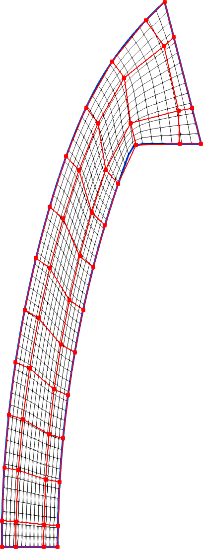
|
(d) Ruled surface |
(e) Control point patch |
(f) Control point patch with control points |
Note that with default settings the blunt-body grid
generated with the Area-orthogonal patch results
in negative cells near the shoulder.
To remedy this, increase the ny value for number
of points in the background grid to get better
resolution of the geometry change around the shoulder.
A nozzle grid

|
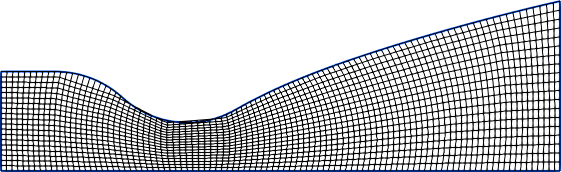
|
(a) Coons patch |
(b) Area-orthogonal patch |
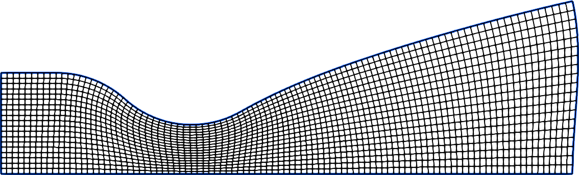
|
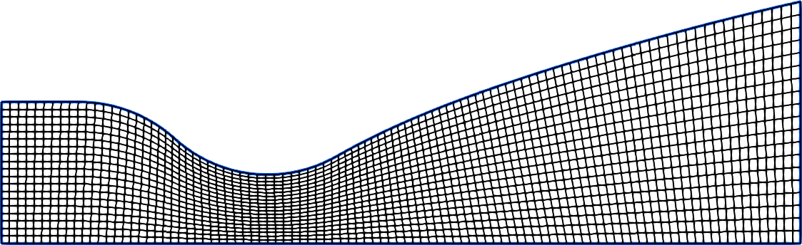
|
(c) Channel patch |
(d) Ruled surface |
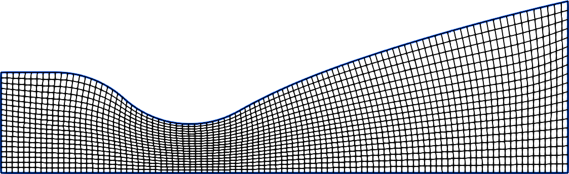
|
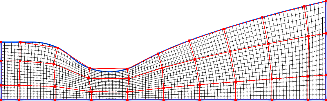
|
(e) Control point patch |
(f) Control point patch with control points |
Here the Area-orthogonal patch with default settings
as cut the corner of the boundary on the nozzle domain.
This behaviour can be improved if some care is take
in selecting the background grid.
We show this here by increasing the
background grid in the x-direction to nx=40
to give a better representation of the change
in geometry in the streamwise direction.
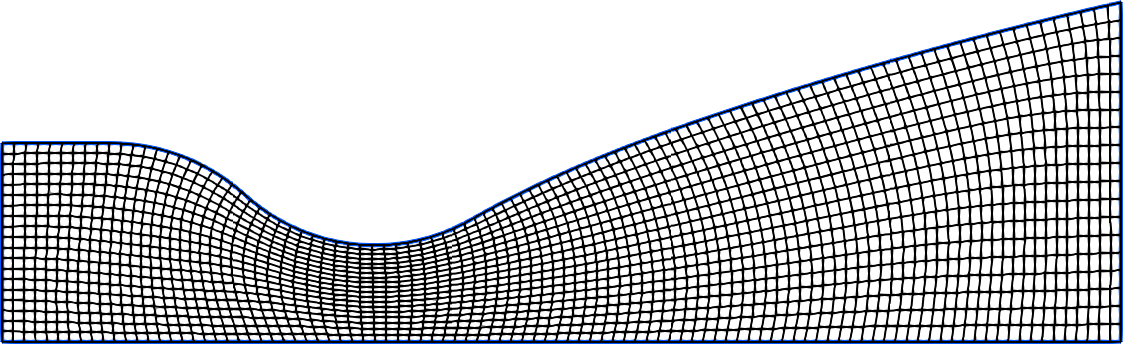
A duct grid
This duct grid mimics the example in Eiseman (1988) A control point form of algebraic grid generation. The channel patch and ruled surface are not appropriate for this domain because the curved boundaries on both the north and east edges. As such, they are not generated for this example.
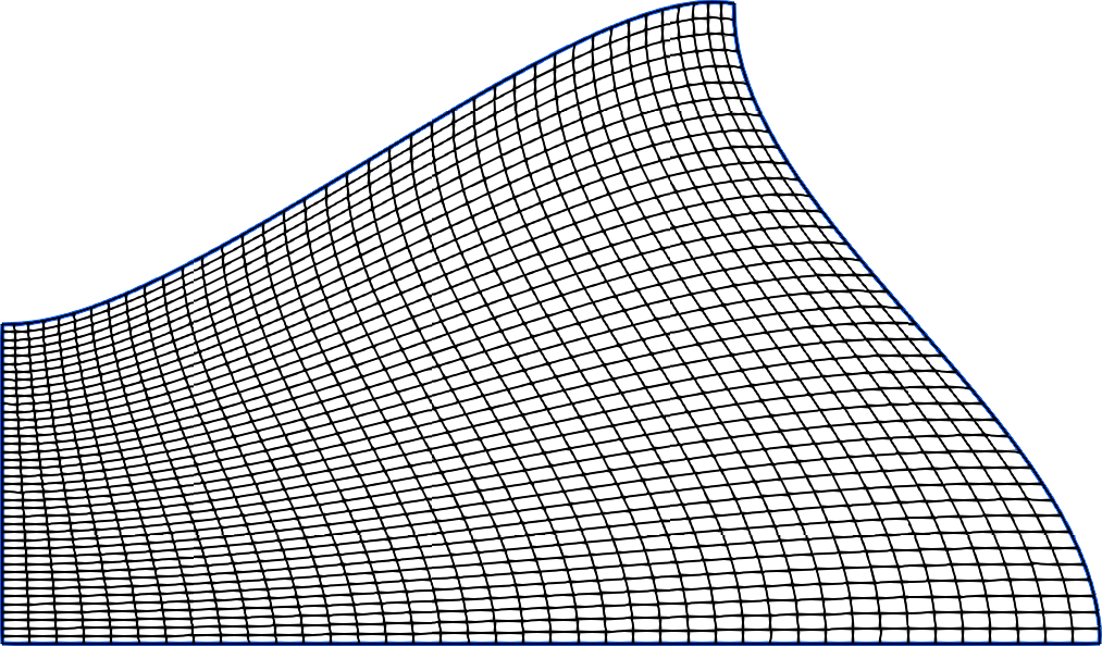
|

|
(a) Coons patch |
(b) Area-orthogonal patch |
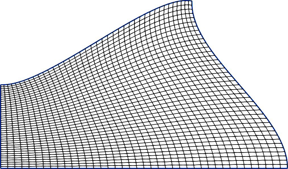
|
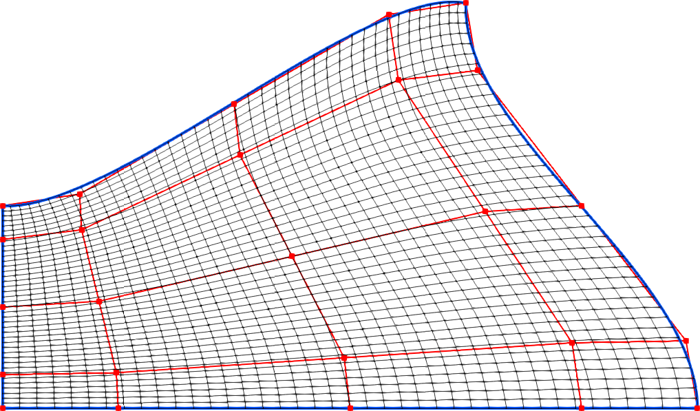
|
(c) Control point patch |
(d) Control point patch with control points |
7.5. Cluster Functions
Cluster Functions are ways of deforming a grid to concentrate the cells in a given area. The most common use for a cluster function is to resolve the boundary layer near a viscous wall, though in hypersonic flow we sometimes cluster near shockwaves as well. Eilmer’s native gridding tool has several cluster functions, a selection of which are documented as follows.
7.5.1. Roberts Function
The Roberts function implmenents a gentle stretching toward a boundary that is controlled by a single parameter beta, which is always greater than one. Closer values to one result in tighter clustering. The two arguments end0 and end1 can be used to indicate which end the clustering should be applied, which can both if required.
This example clusters toward the beginning of a block boundary, with a relatively tight clustering of 1.01:
cf = RobertsFunction:new{end0=true, end1=false, beta=1.01}
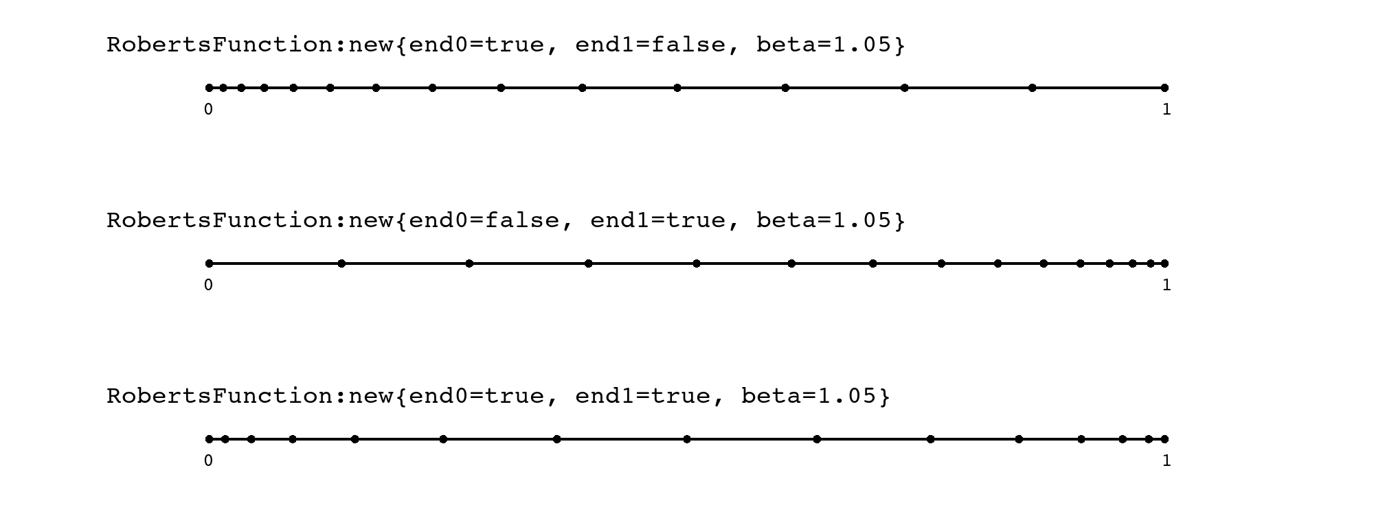
7.5.2. Geometric Function
The geometric function uses a geometric series to grow the cell sizes, starting from a small cell of size a and increasing to a second cell of size ar, then to a third size of ar^2, etc. Eventually, when the cluster function detects that the cells have grown large enough, it switches to a constant cell spacing for the rest of the block. The following example begins with a spacing of one-thousandth the block edge length, and grows by a factor of 1.2 with each step.
cf = GeometricFunction:new{a=0.001, r=1.2, N=60, reverse=false}
Note that the function needs the N argument, which is the number of nodes along the block boundary that is to be clustered, in this case 60. The function also takes a boolean parameter reverse, which can be used to start clustering on the other side of the block.
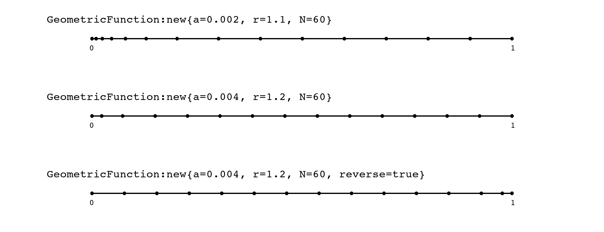
7.5.3. Gaussian Function
The gaussian function applies a bell-curve shaped compression that can be useful for clustering in the middle of a block, perhaps to resolve a shockwave or other feature of interest. The function takes a nondimensional parameter m which can range from 0.0 to 1.0, defining the position of the clustered band; a nondimensional parameter s which defines the width of the band, and a parameter ratio which controls the tightness of the clustering, where smaller numbers are tighter. In the following example, the clustering is positioned at the 80% mark of the block boundary, using a narrow width of 0.2 and a fairly tight ratio of 0.1:
cf = GaussianFunction:new{m=0.8, s=0.1, ratio=0.1}
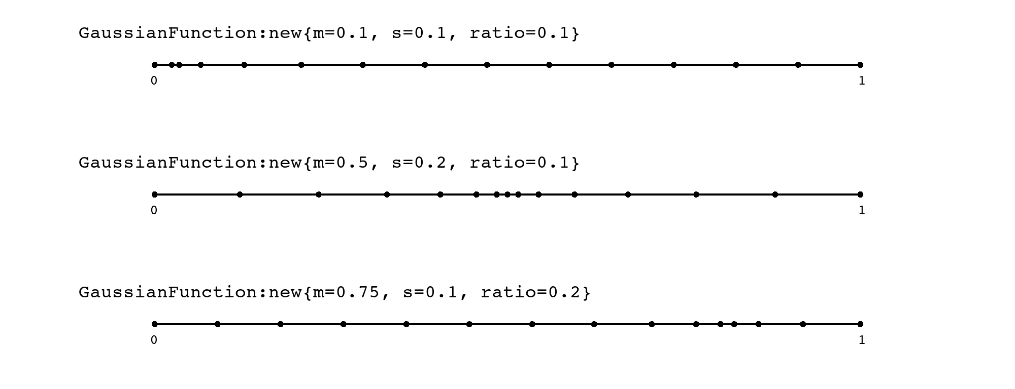
7.5.4. Vinokur Function
The Vinokur function is designed to produce a smooth cell size distribution on an edge which has a constrained cell size at both ends.
The function requires the number of cells on the edge n, the normalised cell size at the start of the edge s0 and the normalised cell size s1 at the end of the edge as arguments.
Note, that the cell sizes are not preserved exactly and can vary significantly, in particular if the cell size varies strongly along the edge.
Should the grid generation fail with an error message saying B<1!, it means that the specified cell sizes are too large to produce a smooth distribution.
Increasing either cell size or reducing the number of cells will solve the problem.
The example below specifies a cell size of ten millionths of the edge length at the start and one millionth of the edge length at its end and a total of 50 cells.
cf = VinokurFunction:new{n=50, s0=1e-5, s1=1e-6}
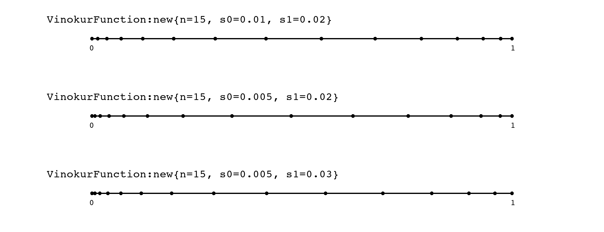
7.5.5. Vinokur-Geometric Function Hybrid
The Vinokur-Geometric Hybrid adds geometric series at either end of the cell distribution and uses the Vinokur function for the cell size distribution in between.
Geometric layers are useful to resolve boundary layers and are specified by a normalised starting cell size, a number of cells and a growth rate.
In the example below, the first cell is one hundred thousandths of the edge length long and cells two to five are larger than their predecessor by a factor of 1.2.
The last cell is one millionths of the edge length long and the nine preceding cells are each larger than the next cell by a factor of 1.1.
This function can also be used to achieve a Vinokur function distribution with exact cell sizes at the ends by setting n0 and r0 to one.
With zero cells in either geometric series the result of the hybrid is the same as the Vinokur function.
cf = VinokurGeomHybridFunction:new{n=50, s0=1e-5, n0=5, r0=1.2, s1=1e-6, n1=10, r1=1.1}
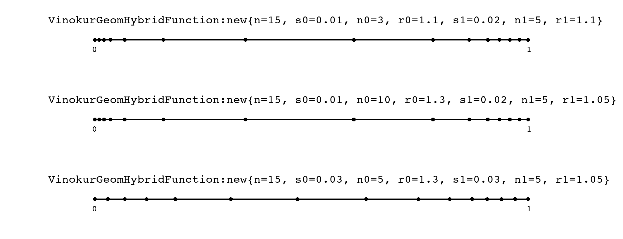
8. Grid objects, methods and functions
8.1. General (for both structured and unstructured grids)
Grid:rotate{rotation_angle=..., rotation_axis=..., [rotation_centre=...]}
This method can be used to rotate the vertices of a grid through an angle about an axis with a specified centre of rotation. If no centre of rotation is provided, the origin is assumed.
rotatation_angle-
float in radians
rotation_axis-
vector given as
Vector3object rotation_centre-
point given as
Vector3object [default:Vector3(0.0, 0.0, 0.0)]
Example: Rotate a structured grid 90 degrees around the y axis.
sg = StructuredGrid:new{...}
theta = math.rad(90)
axis = Vector3:new{x=0.0, y=1.0, z=0.0}
sg:rotate{rotation_angle=theta, rotatation_axis=axis}
Grid:rotate{q=..., [rotation_centre=...]}
This method can be used to rotate vertices of a grid by an amount specified by a unit quaternion with a specified centre of rotation. If no centre of rotation is provided, the origin is assumed.
q-
unit quaternion values as array
{q0, q1, q2, q3}where the unit quaternion is \(q = q_0 + q_1 \hat{i} + q_2 \hat{j} + q_3 \hat{k}\) rotation_centre-
point given as
Vector3object [default:Vector3(0.0, 0.0, 0.0)]
Example: Rotate an unstructured grid 30 degrees around the x-axis direction, with centre of rotation at (0.5, 0.5, 0.5).
usg = UnstructuredGrid:new{...}
theta = math.rad(30)
C = math.cos(theta/2.0)
S = math.sin(theta/2.0)
q = {C, S*1.0, 0.0, 0.0}
usg:rotate{q=q, rotation_centre=Vector3:new{x=0.5, y=0.5, z=0.5}}
8.2. StructuredGrid objects, methods and functions
Here is the list of methods and functions that are specific to structured grids. The more general set of methods and functions that apply to all grids (structured and unstructured) are documented in Grid objects, methods and functions.
StructuredGrid:joinGrid(otherGrid, joinLocation)
Use this method to join another grid onto the current object. If successful, the current object is modified at the end of the operation. It will now contain both grids.
The join grid operation assumes that the edge/face for joining is full-face matching and that the grid points are C0 continuous. The operation does not do extensive checks for badly formed joins. It relies on the caller to use this in a sensible manner.
otherGrid-
second
StructuredGridto be joined joinLocation-
a string specifying at which end of the current grid the other grid should be joined
allowable options are"east","imax","north"and"jmax". Note that the first two are equivalent, and the last two are equivalent.
9. Running a simulation
The overall process of simulation of a gas flow is divided into three stages:
(1) preparation of the defining data,
(2) running the main simulation program, and
(3) postprocessing of the output data from the simulation.
Information is passed from one stage to the next in data files.
9.1. Command-line interface
Eilmer tools and commands are invoked at the command line in the form:
lmr verb [options] [arguments]
To get general help:
$ lmr help
To list all available commands:
$ lmr help -a
Help is available for a specific command:
$ lmr help command-name
9.2. Pre-processing
To start a simulation, we need a gas model, maybe a chemical-kinetics model for reacting flow, simulation configuration and control files, and the initial grid and flow state. Generation of all of these data is the activity of the pre-processing (or preparation) stage.
9.2.1. prep-gas
lmr prep-gas --input=gas-model.lua --output=model.gas

Prepare a gas file for eilmer based on a high-level input file.

required options:
  -i, --input=gasinputfile
      A gas input file, typically a Lua-type input
  -o, --output=gasoutfile
      The name of the output file. This is the file to be used
      by the simulation program. It is the file that appears
      in a setGasModel() call in a simulation input script.

options ([+] can be repeated):
  -v, --verbose [+]
      Increase verbosity during gas file creation.
9.2.2. prep-reactions
lmr prep-reactions [options] --gasfile=model.gas --input=reactions.lua --output=reactions.chem

Prepare a reactions file for eilmer based on a high-level input file.

required options:
  -g, --gasfile=gasmodelfile
      where 'gasmodelfile' has been prepared with the prep-gas command.
      (see: lmr help prep-gas)

  -i, --input=reacinputfile
      where 'reacinputfile' is a Lua-type input that specifies the
      chemical reactions and the parameters for computing rate constants.
      The species that appear in 'reacinputfile' should be consistent
      with the set provided in 'gasmodelfile'.

  -o, --output=reacoutputfile
      where 'reacoutputfile' is the name of the output file. This is the file to be used
      by the simulation program. It is the file that appears when setting 'config.reactions_file'
      in an Eilmer input script.

options ([+] can be repeated):
  -v, --verbose [+]
      Increase verbosity during gas file creation.
  -c, --compact
      Also produce a compact form of the reactions file called 'chem-compact-notation.inp'

For more information on how to construct a 'reacinputfile', see:

      https://gdtk.uqcloud.net/pdfs/reacting-gas-guide.pdf
9.2.3. prep-energy-exchange
lmr prep-energy-exchange [options] --gasfile=model.gas --input=energy-exchange.lua --output=mechanisms.exch [--reacfile=reactions.chem]

Prepare an energy exchange file for eilmer based on a high-level input file.

required options:
  -g, --gasfile=gasmodelfile
      where 'gasmodelfile' has been prepared with the prep-gas command.
      (see: lmr help prep-gas)

  -i, --input=eeinputfile
      where 'eeinputfile' is a Lua-type input that specifies the
      energy exchange mechanisms and the parameters for computing relaxation times.
      The species and energy modes that appear in 'eeinputfile' should be consistent
      with the set provided in 'gasmodelfile'.

  -o, --output=eeoutputfile
      where 'eeoutputfile' is the name of the output file. This is the file to be used
      by the simulation program. It is the file that appears when setting 'config.energy_exchange_file'
      in an Eilmer input script.

options ([+] can be repeated):
  -v, --verbose [+]
      Increase verbosity during gas file creation.
  -r, --reacfile=reacfile
      where 'reacfile' has been prepared with the prep-reactions command (see: lmr help prep-reactions).
      A 'reacfile' is required when there is chemistry coupling specified in the 'eeinputfile'.
9.2.4. prep-grid
lmr prep-grids [options]

Prepare a grid or set of grids based on a file called job.lua.

options ([+] can be repeated):

 -v, --verbose [+]
     Increase verbosity during grid generation.

 -j, --job=grid.lua
     Specify the input file to be different from job.lua.

 --with-cea-usage
     If using a CEAGas in the grid setup script, then the debug-version
     of the executable needs to be called. This flag lets the program know
     in advance that cea will be used, and so the debug executable can be called automatically.
     (Alternatively, one could call 'lmr-debug' directly at prep grid stage.)
9.2.5. prep-sim
lmr prep-sim [options]

Prepare an initial flow field and simulation parameters based on a file called job.lua.

options ([+] can be repeated):

 -v, --verbose [+]
     Increase verbosity during preparation of the simulation files.

 -j, --job=flow.lua
     Specify the input file to be something other than job.lua.
     default: job.luare

 --with-cea-usage
     If using a CEAGas as part of the simulation setup, then the debug-version
     of the executable needs to be called. This flag lets the program know
     in advance that cea will be used, and so the debug executable can be called automatically.
     (Alternatively, one could call 'lmr-debug' directly at prep stage.)
9.3. Run-time
Now that the initial flow and grid files exist, it is time to run the main
flow simulation process.
By default, four executables are built:
lmr-run, lmrZ-run, lmr-mpi-run and lmrZ-mpi-run.
The Z variants use complex values; the others use real values.
For shared memory, the user can call lmr run and the launcher will figure out the best executable to call based on whether one is running transient or steady.
For running with MPI, things are a bit trickier because we need to play nicely with the MPI launcher.
We recommend using lmr-mpi-run for most transient simulations and lmrZ-mpi-run for steady mode.
9.3.1. run
lmr run [options]

Run an Eilmer simulation.

When invoking this command, the shared memory model of execution is used.
This command assumes that a simulation has been pre-processed
and is available in the working directory.

For distributed memory (using MPI), use the stand-alone executable 'lmr-mpi-run'.
For example:

   $ mpirun -np 4 lmr-mpi-run

options ([+] can be repeated):

 -s, --snapshot-start
     Index of snapshot to use when starting iterations.
     examples:
       -s 1 : start from snapshot 1
       --snapshot-start=3 : start from snapshot 3
       -s -1 : start from final snapshot
       -s=0 : (special case) start from initial condition
     default: none

     NOTE: if the requested snapshot index is greater than
           number of snapshots available, then the iterations will
           begin from the final snapshot.

 --start-with-cfl <or>
 --cfl
     Override the starting CFL on the command line.

     --start-with-cfl=100 : start stepping with cfl of 100
     --cfl 3.5 : start stepping with cfl of 3.5
     default: no override

     NOTE: When not set, the starting CFL comes from input file
           or is computed for the case of a restart.

 --max-cpus=<int>
     Sets maximum number of CPUs for shared-memory parallelism.
     default: 64 (on this machine)

     NOTE: in solver_mode=steady, this option has no effect.

 --threads-per-mpi-task=<int>
     Sets threads for MPI tasks when running in MPI mode.
     Leave the default value at 1 unless you know what you're doing
     and know about the distributed/shared memory parallel processing
     model used in Eilmer.
     default: 1

     NOTE: in solver_mode=steady, this option has no effect.

 --max-wall-clock=hh:mm:ss
     This the maximum simulation duration given in hours, minutes and seconds.
     default: 24:00:00
 <OR>
 --max-wall-clock=s
     A single integer value in seconds can also be given.
     A value of -1 disables the max-wall-clock stopping criterion.


 -v, --verbose [+]
     Increase verbosity during progression of the simulation.
9.4. Command and control during run-time
There could be several reasons one might like to interrupt the normal flow of a simulation to request an action.
Some examples are: adjust a CFL value; request a current snapshot of the simulation evolution; or stop a simulation early.
The facility to interrupt and act during a simulation is provided by user-edited files.
We have two separate files for steady mode and transient mode because the kinds of actions available differ
(and due to historical reasons).
In general, these files are re-read at specific step intervals.
If an action is detected at one of the checking intervals, it is executed.
When issuing run-time command and control decisions, there is a trade-off between reproducibility and "getting things done". In terms of reproducibility, you weaken the record of your simulation settings if you adjust values on-the-fly. You can mitigate this by keeping good notes in your workbook, and we try to record the actions executed at run-time to STDOUT. That being said, you might be interested in a one-time simulation and it’s handy to be able to adjust how the simulation proceeds without stopping and restarting. This can be particularly handy if you have a long-run job (eg. 6—12 hours) on a cluster computer and don’t want to re-queue.
9.4.1. Issuing run-time commands to steady-state solver (config.solver_mode = "steady")
Users can issue run-time commands to the solver in steady mode by editing the file:
lmrsim/commands-to-steady-mode
Here is an example file. This particular example does nothing to alter the run-time behaviour of the simulation since the actions are disabled.
write-snapshot:
  at-next-check: no
  at-next-check-after-step: -1

stop:
  at-next-check: no
  at-next-check-after-step: -1
The configuration controlling how often the commands file is read is
part of the Newton-Krylov settings. It is: steps_between_command_updates.
The default is 10 steps.
There is a performance cost to the simulation to read and execute commands,
so make an appropriate selection.
If you have a large simulation running on a cluster computer and the cost
per iteration is on the order of minutes, then steps_between_command_updates = 1 might be useful to you.
That cost of reading the file is small compared to the step update.
On the other hand, for a simulation that runs in seconds and you want to do many as part of a parameter sweep, you might find you do not want the cost of reading the commands file.
In that case, set the steps_between_command_updates to a value larger than your maximum steps.
Commands are in the form of what and when.
There are currently two what commands: write-snapshot and stop.
write-snapshot-
writes a snapshot in next slot in the snapshot sequence
stop-
stops the simulation cleanly (but does not necessarily write-on-exit; use in conjuction with
write-snapshotto achieve a write-on-exit)
In terms of when, there are two options:
at-next-check-
boolean, yes|no
perform the action next time the commands file is read at-next-check-after-step-
int,
step number
perform the action at the next check when current step exceeds step number, but don’t repeat action untilstep numberis changed
if set to -1, this is disabled.
Example:steps_between_command_updatesis set to 10 andat-next-check-after-stepis set to 15.
For these settings, the action is performed at step 20. The checks occur at steps: 10, 20, 30, … When check occurs at step 20, thencurrent step > step number→20 > 15. This is the next check that occurred that satisfied the condition, so the action is performed.
There is a priority order given to the commands. That order is:
-
Writing commands
-
Stop commands
So if you want to write and exit, you can set at-next-check to yes for
both the write and stop commands.
9.4.2. Controlling the time-marching mode at run-time (config.solver_mode = "transient")
See lmrsim/control file.
9.5. Post-processing
The Eilmer flow field data is a native format. We will typically need to process it in some way to make is usable for analysis or visualisation. Here are some of the Eilmer tools that can be used as a part of your post-processing.
9.5.1. snapshot2vtk
lmr snapshot2vtk [options]

Convert a flow field using one or more snapshots to VTK format.

If no options related to snapshot selection are given,
then the default is to process the final snapshot.

options ([+] can be repeated):

 -s, --snapshot[s]+
     comma separated array of snapshots to convert
     examples:
       --snapshots=0,1,5 : processes snapshots 0, 1 and 5
       --snapshot=2 : processes snapshot 2 only
       --snapshot 1  --snapshot 4 : processes snapshots 1 and 4
     default: none (empty array)


 -f, --final
     process the final snapshot
     default: false

 -a, --all
     process all snapshots
     default: false

 -b, --binary-format
     selects binary format for output
     default: false

 --add-vars
     comma separated array of auxiliary variables to add in VTK
     eg. --add-vars="mach,pitot"
     Other variables include:
         total-h, total-p, total-T,
         enthalpy, entropy, molef, conc,
         Tvib (for some gas models)
         nrf (non-rotating-frame velocities)
         cyl (cylindrical coordinates: r, theta)

 -r, --subtract-ref-solution
     name of file containing a Lua-format reference solution
     matching field variables in solution files and reference solution
     will be altered as: numerical value - reference value
     examples:
     --subtract-ref-solution=ref-soln.lua
     default: none

 --subtract-solid-ref-solution
     name of file containing a Lua-format reference solution for the solid domains
     matching field variables in solution files and reference solution
     will be altered as: numerical value - reference value
     examples:
     --subtract-solid-ref-solution=solid-ref-soln.lua
     default: none

 -v, --verbose [+]
     Increase verbosity during preparation and writing of VTK files.
9.5.2. probe-flow
lmr probe-flow [options]

Probe flow-field snapshots based on a selection of field variables.

If no selection of variable names is supplied, then the default action is
to probe all flow field variables (--names=all).

If no options related to snapshot selection are given,
then the default is to process the final snapshot.

options ([+] can be repeated):

 -n, --names
     comma separated list of variable names for reporting
     examples:
       --names=rho,vel.x,vel.y
       --names=rho
     default:
       --names=all

 --add-vars
     comma separated array of auxiliary variables to add to the flow solution
     eg. --add-vars=mach,pitot
     Other variables include:
         total-h, total-p, total-T,
         enthalpy, entropy, molef, conc,
         Tvib (for some gas models)
         nrf (non-rotating-frame velocities)
         cyl (cylindrical coordinates: r, theta)

 -l, --location
     probes the flow field at locations 0, 1 and 2 by accepting a string of the form
     "x0,y0,z0;x1,y1,z1;x2,y2,z2"

     For 2D, simply supply 0 for z, or omit.
     To avoid the shell cutting your command at the semicolon, use quotes.
     example:
       --location="0.25,0.25,0.0;0.75,0.75"

     default: none (report nothing)

 -s, --snapshot[s]+
     comma separated array of snapshots to convert
     examples:
       --snapshots=0,1,5 : processes snapshots 0, 1 and 5
       --snapshot=2 : processes snapshot 2 only
       --snapshot 1  --snapshot 4 : processes snapshots 1 and 4
     default: none (empty array)

 -f, --final
     process the final snapshot
     default: false

 -a, --all
     process all snapshots
     default: false

 -o, --output
     write output to a file
     example:
       --output=norms-data.txt
     default: none (just write to STDOUT)

 -v, --verbose [+]
     Increase verbosity.
9.5.3. slice-flow
lmr slice-flow [options]

Slice flow-field snapshots across index-directions,
for a selection of flow field variables.
The really only makes sense for structured-grid blocks.

If no selection of variable names is supplied, then the default action is
to report all flow field variables (--names=all).

If no options related to snapshot selection are given,
then the default is to process the final snapshot.

options ([+] can be repeated):

 -n, --names
     comma separated list of variable names for reporting
     examples:
       --names=rho,vel.x,vel.y
       --names=rho
     default:
       --names=all
     The output will always start with pos.x,pos.y and, for 3D, pos.z.

 --add-vars
     comma separated array of auxiliary variables to add to the flow solution
     eg. --add-vars=mach,pitot
     Other variables include:
         total-h, total-p, total-T,
         enthalpy, entropy, molef, conc,
         Tvib (for some gas models)
         nrf (non-rotating-frame velocities)
         cyl (cylindrical coordinates: r, theta)

 -l, --slice-list
     slices the flow field in a range of blocks by accepting a string of the form
     "blk-range,i-range,j-range:k-range;"

     examples:
       --slice-list=0:2,:,$,0
       will select blocks 0 and 1, writing out the top strip (j=njc-1) of cells, stepping in i
       Note that you can specify the last value of any index with $.

       --slice-list="0:2,:,0,0;2,$,:,0"
       will select blocks 0 and 1, writing out a strip of cells stepping in i, keeping j=0, k=0, plus
       from block 2, write out a strip of cells stepping in j, keeping i=nic-1 and k=0
       Note that you need the quotes to stop the shell from cutting your command at the semicolon.

     default: none (report nothing)

 -s, --snapshot[s]+
     comma separated array of snapshots to convert
     Note that only the last one will be processed.
     examples:
       --snapshots=0,1,5 : processes snapshots 0, 1 and 5
       --snapshot=2 : processes snapshot 2 only
       --snapshot 1  --snapshot 4 : processes snapshots 1 and 4
     default: none (empty array)


 -f, --final
     process the final snapshot
     default: false

 -a, --all
     process all snapshots
     default: false

 -o, --output
     write output to a file
     example:
       --output=norms-data.txt
     default: none (just write to STDOUT)

 -v, --verbose [+]
     Increase verbosity.
9.5.4. extract-line
lmr extract-line [options]

Extract lines of data from flow-field snapshots,
for a selection of flow field variables.
Works on structured-grid and unstructured-grid blocks.

If no selection of variable names is supplied, then the default action is
to report all flow field variables (--names=all).

If no options related to snapshot selection are given,
then the default is to process the final snapshot.

options ([+] can be repeated):

 -n, --names
     comma separated list of variable names for reporting
     examples:
       --names=rho,vel.x,vel.y
       --names=rho
     default:
       --names=all
     The output will always start with pos.x,pos.y and, for 3D, pos.z.

 --add-vars
     comma separated array of auxiliary variables to add to the flow solution
     eg. --add-vars=mach,pitot
     Other variables include:
         total-h, total-p, total-T,
         enthalpy, entropy, molef, conc,
         Tvib (for some gas models)
         nrf (non-rotating-frame velocities)
         cyl (cylindrical coordinates: r, theta)

 -l, --line-list
     lines from point 0 to point 1 and sample numbers are specified as a string of the form
     "x0,y0,z0,x1,y1,z1,n;"
     Note that you need the quotes to stop the shell from cutting your command at the semicolon.
     default: none (report nothing)

 -s, --snapshot[s]+
     comma separated array of snapshots to convert
     Note that only the last one will be processed.
     examples:
       --snapshots=0,1,5 : processes snapshots 0, 1 and 5
       --snapshot=2 : processes snapshot 2 only
       --snapshot 1  --snapshot 4 : processes snapshots 1 and 4
     default: none (empty array)


 -f, --final
     process the final snapshot
     default: false

 -a, --all
     process all snapshots
     default: false

 -o, --output
     write output to a file
     example:
       --output=norms-data.txt
     default: none (just write to STDOUT)

 -v, --verbose [+]
     Increase verbosity.
9.5.5. compute-norms
lmr compute-norms [options]

Compute norms for a snapshot based on selection of field variables.

If a reference solution provided (as Lua file), then use that to compute error norms for
selected field variables.

If no selection of norm variables is supplied, then the default action is
to compute a density norm (--norms="rho").

If no options related to snapshot selection are given,
then the default is to process the final snapshot.

options ([+] can be repeated):

 -n, --norms
     comma separated list of variables for norms calculation
     examples:
       --norms="rho,velx,vely"
       --norms="rho"
     default:
       --norms="rho"
       If no norms-list supplied, then just process density.

 --solid-norms
     comma separated list of variables for norms calculation in solid domains
     examples:
       --solid-norms="T,e"
     default: none (don't do anything for solid domain)

 -r, --reference-solution
     a reference solution provided in a Lua file

     the reference solution will be subtracted from the field variables
     depending on which variables are provided in the reference solution

     examples:
       --reference-solution=my_ref_soln.lua
       -r ref-solution.lua
     default: none (just compute field norms)

 --limit-to-region
     limits the norm computation to a box with lower corner (x0,y0,z0)
     and upper corner (x1,y1,z1) by accepting a string of the form
     "x0,y0,z0,x1,y1,z1"

     this is sometimes useful to focus the error estimate on the interior
     away from boundaries

     for 2D, simply supply z = 0.0 for z0 and z1
     examples:
       --limit-to-region="0.25,0.25,0.0,0.75,0.75,0.0"

     default: none (just use entire domain)

 -s, --snapshot[s]+
     comma separated array of snapshots to convert
     examples:
       --snapshots=0,1,5 : processes snapshots 0, 1 and 5
       --snapshot=2 : processes snapshot 2 only
       --snapshot 1  --snapshot 4 : processes snapshots 1 and 4
     default: none (empty array)


 -f, --final
     process the final snapshot
     default: false

 -a, --all
     process all snapshots
     default: false

 -o, --output
     write output to a file
     example:
       --output=norms-data.txt
     default: none (just write to STDOUT)

 -v, --verbose [+]
     Increase verbosity.
10. Warnings
Eilmer may emit various warnings at preparation stage or at run time. These warnings will usually say what it thinks is awry and a suggested fix. The warnings don’t really explain the reasoning behind it due to screen real estate and avoiding overloading the user. The explanations might be nuanced. Here in the reference manual, we attempt to give more information.
Warning 00: use-of-extrema-clipping-
If aiming for deep convergence with a steady-state simulation, the use of
extrema_clippingis often an interference. We can state this more generally: the use of clips and switches are a hindrance to deep convergence.At the local level of a cell, the flow conditions might sit just on the edge of a clip or switch value. If on the next iteration, that value falls on the other side, then a clip or switch is engaged. When far from convergence, this is not an issue. When close to convergence, the switching/clipping behaviour is "shifting the rug" so to speak on the flow field state. This will often result in a ringing for the residual.
The
extrema_clippingflag falls into this category of clips. The recommendation for steady-state simulations is:config.extrema_clipping = false