Control Point Form Grid Generation
Caiyu (Carrie) Xie and Rowan J. Gollan, 2021-12-19
Control point form grid generation is an algebraic technique to produce structured grids. It is more powerful than transfinite interpolation because it makes use of internal control points to give more control on the grid point distribution. By contrast, a transfinite interpolated grid is completely specified by the boundaries. The extra control comes at the cost of more input required by the user. This note documents the background mathematics and gives examples of user input in terms of control points so that you may see the resulting structured grids.
1. Control point formulation in two dimensions 1
Equations 1 and 2 below are used to generate horizontal and vertical gridlines. The range of horizontal parameter r is [1, N-1]; the range of vertical parameter s is [1, M-1], where N is the number of control points in horizontal direction (i = 1, 2, …, N), and M is the number of control points in vertical direction (j = 1, 2, …, M). The transformation from \(r \in [1,N]\) and \(s \in [1,M]\) to \(\hat{r},\hat{s} \in [0,1]\) has been taken care of in Eilmer. \(G_{\alpha}(r)\) and \(H_{\beta}(s)\) are the integration functions.
Having either \(E_{j}(r)\) or \(F_{i}(s)\) function, the tensor product form can be produced:
or
To ensure the grid conforms precisely to prescribed boundaries, the Boolean sum is used. P(1,s), P(N-1,s), P(r,1) and P(r,M-1) in Equation 5 are the west, east, south and north boundary, respectively.
2. Usage of ControlPointPatch
ControlPointPatch:new{south=pathS, north=pathN, west=pathW, east=pathE,
control_points=ctrl_pts}
: a control point form surface between the four pathes. The orientation of Path elements
is important. The north and south boundaries progress west to east, and west and east boundaries progress south to
north.
The control points are stored in a 2D array. The structure of ctrl_pts should be an array of columns of control points.
In the Lua file, ctrl_pts[i][j] gives the control point in \(i^{th}\) column and \(j^{th}\) row.
The control points progress from south to north vertically and west to east horizontally. The boundary control points do
not have to lie on prescribed boundaries.
If uniform grid is desired, interior control points should be uniformly distributed, and boundary control points should be half of the unit spacing from the control points directly adjacent to them. Therefore, the unit spacings in r and s directions are \(L/(N-2)\) and \(H/(M-2)\), respectively, where L and H are length and height of the grid.
3. Examples of using ControlPointPatch
3.1. Generate grid for a unit square
The ctrl_pts is defined as an array of columns of control points.
L = 1.0
N = 4
M = 5
ctrl_pts = {}
xPos = {0.0, L/4, 3*L/4, L}
yPos = {0.0, L/6, 3*L/6, 5*L/6, L}
for i=1,N do
   ctrl_pts[i] = {}
   for j=1,M do
      ctrl_pts[i][j] = Vector3:new{x=xPos[i], y=yPos[j]}
   end
end
The south, north, west and east boundaries are defined by Paths.
south = Line:new{p0=ctrl_pts[1][1], p1=ctrl_pts[N][1]}
north = Line:new{p0=ctrl_pts[1][M], p1=ctrl_pts[N][M]}
west = Line:new{p0=ctrl_pts[1][1], p1=ctrl_pts[1][M]}
east = Line:new{p0=ctrl_pts[N][1], p1=ctrl_pts[N][M]}
The control point surface and grid can be generated as follows.
ctrlPtPatch = ControlPointPatch:new{north=north, east=east, west=west, south=south, control_points=ctrl_pts}
grid = StructuredGrid:new{psurface=ctrlPtPatch, niv=21, njv=21}
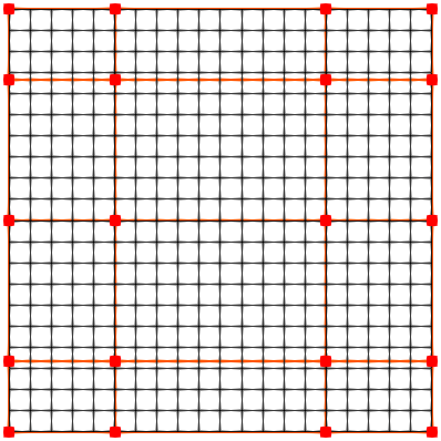
The corresponding grid is shown in Figure 1 (control points and control net in red, gridlines in black).
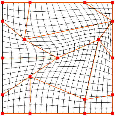
3.2. Move internal points
Gridlines can be adjusted flexibly by moving internal control points. This example shows the same unit square with modified internal control points. The new control points locations are:
ctrl_pts[2][2] = Vector3:new{x=xPos[2],y=L/3}
ctrl_pts[2][3] = Vector3:new{x=L/2,y=yPos[3]}
ctrl_pts[2][4] = Vector3:new{x=L/5,y=2*L/3}
ctrl_pts[3][2] = Vector3:new{x=xPos[3],y=L/8}
ctrl_pts[3][3] = Vector3:new{x=3.5*L/4,y=2*L/3}
ctrl_pts[3][4] = Vector3:new{x=xPos[4],y=2.5*L/3}
The resulting grid is displayed in Figure 2.
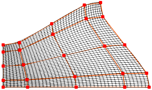
3.3. Reproduce the duct grid in Eiseman’s paper 1
Exact boundaries of the duct grid are not given in the paper, so some estimations are used.
The north and east boundary paths are determined using Bezier curves. The west and south boundary paths are defined by Line object.
The control points adjacent to boundaries have half of the unit spacings between them and the control points at boundaries to get uniform grid.
--x coordinates of control points on east boundary (5x5 control points)
L0 = 12
L1 = 11.8
L2 = 10
L3 = 8.2
L4 = 8

--y coordinates of control points on north boundary (5x5 control points)
H0 = 3.5
H1 = 3.7
H2 = 5.25
H3 = 6.8
H4 = 7

N = 5
M = 5

L={L0,L1,L2,L3,L4}
H={H0,H1,H2,H3,H4}

-- To ensure uniform distribution of coordinate curves,
-- the control points adjacent to boundaries have increments of half unit spacing.
-- x = C*(L/(N-2); y = D*(H/(M-2))
-- The function coeff(index,N) is used to compute coefficients C and D
function coeff(index,N)
   if index == 1 then return 0
   elseif index == 2 then return 0.5
   elseif index == N then return N-2
   else return index-1.5
   end
end

-- unit spacing of each horizontal line
usx={}
for j=1,M do
   usx[j] = L[j]/(N-2)
end

-- unit spacing of each vertical line
usy={}
for i=1,N do
   usy[i] = H[i]/(M-2)
end

-- Compute and store coefficients in vertical direction
cj={}
for j = 1,M do
   cj[j]=coeff(j,M)
end

-- Locate each control point
ctrl_pts = {}
for i=1,N do
   ctrl_pts[i] = {}
   -- Compute coefficient in horizontal direction
   ci = coeff(i,N)
   for j=1,M do
      ctrl_pts[i][j]=Vector3:new{x=ci*usx[j],y=cj[j]*usy[i]}
   end
end

-- west straight line boundary
west = Line:new{p0=ctrl_pts[1][1],p1=ctrl_pts[1][M]}

-- north Bezier boundary
n0 = ctrl_pts[1][M]
n1 = Vector3:new{x=ctrl_pts[2][M-1].x,y=(M-2.25)*usy[2]}
n2 = ctrl_pts[math.ceil(N/2)][M]
n3 = Vector3:new{x=ctrl_pts[N-1][M].x,y=(M-1.8)*usy[N-1]}
n4 = ctrl_pts[N][M]
north = Bezier:new{points={n0,n1,n2,n3,n4}}

-- east Bezier boundary
e0 = ctrl_pts[N][1]
e1 = Vector3:new{x=(N-1.95)*usx[2],y=0.75*usy[N]}
e2 = ctrl_pts[N][math.ceil(M/2)]
e3 = Vector3:new{x=(N-2.1)*usx[M-1],y=(N-2.75)*usy[N]}
e4 = ctrl_pts[N][M]
east = Bezier:new{points={e0,e1,e2,e3,e4}}

--south straight line boundary
south =  Line:new{p0=ctrl_pts[1][1],p1=ctrl_pts[N][1]}

ctrlPtPatch = ControlPointPatch:new{north=north, east=east, west=west, south=south, control_points=ctrl_pts}

grid = StructuredGrid:new{psurface=ctrlPtPatch, niv=41, njv=41}
grid:write_to_vtk_file('duct-grid.vtk')
The duct grid with its control points and net is shown in Figure 3.
Reference
-
[1] Eiseman, Peter R. (1988). A control point form of algebraic grid generation. International Journal for Numerical Methods in Fluids, vol 8, pp 1165—1181. https://doi.org/10.1002/fld.1650081005