Hybrid fluxes, shock detection and smoothing
Daryl M. Bond, 2021-09-07
1. Adaptive flux calculation
We often want to capture flow features that require low dissipation numerical methods to resolve and yet also contain discontinuities that these schemes struggle to handle in a stable manner. One way of addressing this issue is to use adaptive flux solvers which combine two different (but compatible) ways of calculating the inviscid fluxes, typically a low dissipation but sensitive solver and the other a highly dissipative but stable solver, and then select some combination of the two in order to best achieve our requirements. This can be represented according to,
\(F=SF_{A}+\left(1-S\right)F_{B}\)
where \(F\) is the final flux, \(0\leq S\leq1\) is a blending variable, and \(F_{A}\) and \(F_{B}\) are the two fluxes that are being blended. From this we can see that \(F\) can be equal to \(F_{A}\), \(F_{B}\), or some linear combination of the two. So, now we have a way of selecting which flux or combination thereof that we would like to use at any interface in our domain, we simply need to detect where our discontinuities are located and ensure that in those regions we have our stability maintaining high-dissipation flux calculator turned on. Meanwhile, elsewhere in the domain, we want to ensure that we are using the low dissipation flux so that we can capture as much of the physics as possible.
2. Shock detection
The problem of detecting discontinuities is a challenging one and is an active area of research. In Eilmer 4 we currently provide a single function for shock detection that checks for compression and shear at an interface and compares these values to some user defined threshold values. This approach results in our shock detector value, or flux blending variable, S having a value of 0 or 1 and can be seen in the figure below, where the compression and shear tolerances are -0.1 and 1.0, respectively.
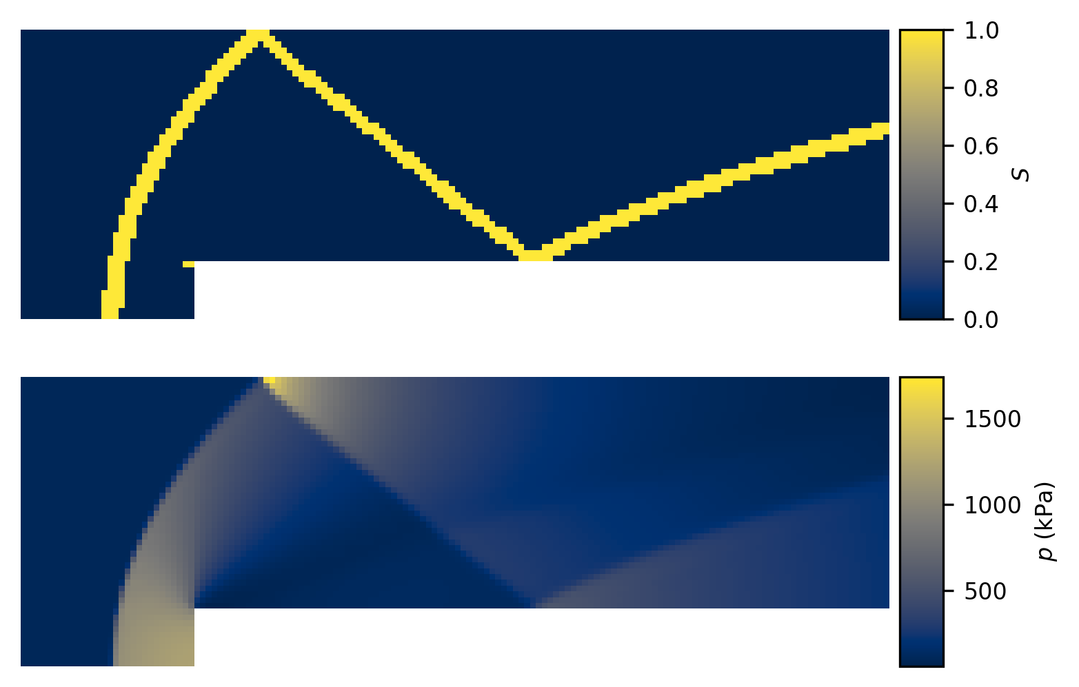
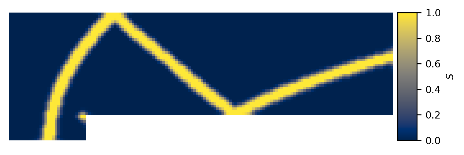
From this figure it is clear that we are mostly capturing the shocks, but are doing so in a manner that introduces sharp transitions between our selected flux calculators. Having sharp transitions can introduce spurious oscillations into the flow field and so we would prefer to have a smooth transition. This can be achieved by calculating our variable S in such a way that it smoothly varies from zero to one, depending on the local flow conditions, or we can apply a post-processing step to spatially diffuse a binary shock detector. Eilmer 4 has the second option implemented where S is spatially averaged as part of an iterative process where information is propagated through faces and cells, as described in the algorithm below. Note that any cell that is initially marked as a definite discontinuity, that is with S=1, is never modified. Indeed, it can be seen that the averaging process treats these points as a constant source that sustains the growth of the averaging wave-front. The result of aplying smoothing can be seen in the following figure where three averaging iterations have been performed.
compute S for all faces
set S in each cell to maximum of connected faces
for each averaging iteration
  for each face
    set face S to maximum of left and right cell
  end
  for each cell
    if cell S=1 continue
    set cell S to average of connected faces
  end
end

set S in each face to maximum of left and right cell
3. Practical considerations
In order to use the smoothing feature the user will need to know a number of configuration options:
config.flux_calculator-
string, default:
'adaptive_hanel_ausmdv'
If a hybrid flux is desired then it must be specified here. These are identified by the use of `adaptive' in their names. config.shock_detector_smoothing-
int, default:
0
This determines the number of averaging or smoothing iterations that are carried out. Note that each iteration requires inter-block communication and so it is somewhat expensive. The default is zero and so no smoothing takes place. config.strict_shock_detector-
boolean, default:
true
If this is true then any face that is part of a cell with S>0 will have its own S value set to 1. This is to emulate legacy behaviour and thus defaults to true. For true blending of fluxes this should be set to false.