Catalogue of Examples
In the source tree for Eilmer, there are a number of examples of the simulation code in action. These examples have been collected and maintained over many years. Some are well-tested and exercised, while others are more bleeding edge. The hope is that all of the examples offer launching points for you to start your own compressible flow simulations.
A number of these examples replicate classic test cases in the CFD literature on compressible flows, or classic experiments in high-speed flow. The listing below provides a mapping directories in the source tree to the literature. They are grouped loosely by the type of flow/geometry configuration. This is not a perfect grouping because the world of compressible flow test cases is not always so easy to categorise.
1. External, inviscid flows of perfect gases
1.1. 2D/foil-circular-arc-transonic
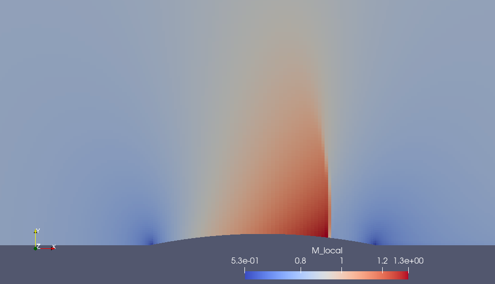
This example shows the transonic flow around an airfoil with a circular-arc profile. It appears to be a standard example in the textbooks on Computational Fluid Dynamics, where the solution for the full potential equations are discussed. Note that, effectively, the Euler equations solved here. Also, the image does not show the complete flow domain used for the simulation. The upper boundary is 6 chord lengths above the lower boundary and the inlet and outlet boundaries are each 5 chord lengths from the airfoil.
1.2. 2D/sphere-lehr/m355

This shock-fitting example shows the transient flow of a hydrogen/oxygen gas mixture over a spherical projectile. The test case is derived from the experiments by Lehr (1972) with conditions corresponding to Figure 5 of his original paper. The glyphs overlaid on the animation are points manually digitized from the shock front in that figure.
Reference:
-
Hartmuth F. Lehr. (1972),
Experiments on Shock-Induced Combustion,
Acta Astronautica, 17, pp.589—597
2. Internal, inviscid flows of perfect gases
2.1. 2D/nozzle-conical-back
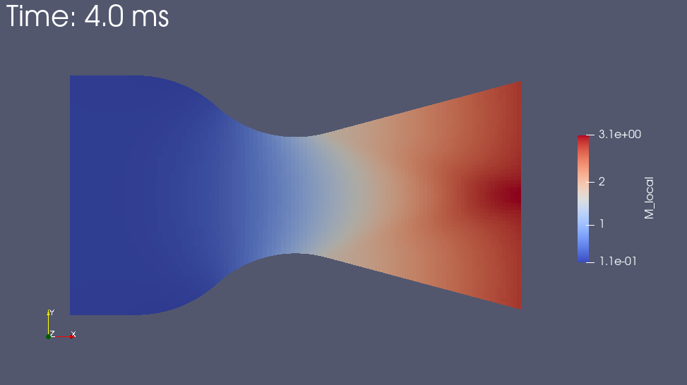
This example shows the acceleration of gas through a converving-diverging nozzle. The left boundary is subsonic and driven by the stagnation condition of a hypothetical reservoir. The case is interesting because there are experimentally-measured wall pressures for the supersonic part of the nozzle.
Reference:
-
LH Back, PF Massier and HL Gier (1965),
Comparison of measured and predicted flows through conical supersonic nozzles, with emphasis on the transonic region.
A.I.A.A. Journal 3(9): pp.1606-1614.
2.2. 2D/forward-facing-step
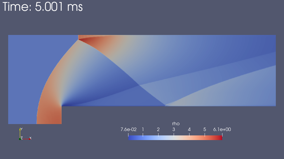
This example shows the flow of gas at Mach 3 over a forward-facing step in a duct. The test case was first proposed by Emery (1968) and is described as a two-dimensional step. However, in the literature, this test case is often cited for its use in the paper by Woodward and Colella (1984) which tested the capabilities of various difference schemes for treating strong shocks. They describe this case as a Mach 3 Wind Tunnel with a Step.
References:
-
Emery (1968),
An Evaluation of Several Differencing Methods for Inviscid Fluid Flow Problems,
Journal of Computational Physics, 2: pp.306-331. -
Woodward and Colella (1984),
The Numerical Simulation of Two-Dimensional Fluid Flow with Strong Shocks,
Journal of Computational Physics, 54: pp.115-173.
2.3. 2D/richtmyer-meshkov

This example consists of a curved interface between two fluids of different density that is processed by a shock passing left to right through the domain. The misaligned density gradient at the interface and pressure gradient at the shock induce a symmetric swirling motion of the interface, which is driven by the baroclinic production of vorticity during the impact. This vorticity is visualised in the colourmaps as blue for clockwise (negative) swirling motion and red for anti-clockwise (positive) motion, overlayed on a greyscale map describing the temperature. As the simulation progresses, the interface grows unstably into a complex structure consisting of a "spike" of cold fluid piercing leftward, and a "bubble" of hot fluid on the right. In the simulation these structures convect out of the domain within 200 ms, but with more time a turbulent interface would form, with both spike and bubble decaying into a random chaotic mess.
The first theoretical description of this kind of instability was given by the American physicist Robert D. Richtmyer in 1960, followed by experimental results published in 1969 by the Russian physicist Evgeny Meshkov. The phenomenon of unstable growth of a density interface due to shock compression is named the Richtmyer-Meshkov instability (RMI) in recognition of their efforts.
The Richtmyer-Meshkov instability plays a role in many flows of engineering and scientific interest. In inertial confinement fusion it is responsible for mixing the hot target material into the colder surroundings, reducing fusion yield and making positive net energy production more difficult. Conversely, in high speed aircraft engines shock induced mixing is employed deliberately to help mix fuel and air, accelerating combustion and leading to greater engine performance.
-
Robert D. Richtmyer (1960),
Taylor instability in shock acceleration of compressible fluids,
Communications on Pure and Applied Mathematics, 13(2). -
E. E. Meshkov (1969),
Instability of the interface of two gases accelerated by a shock wave,
Fluid Dynamics, 4(101-104).
3. Jets and shear layers
3.1. 2D/underexpanded-jet
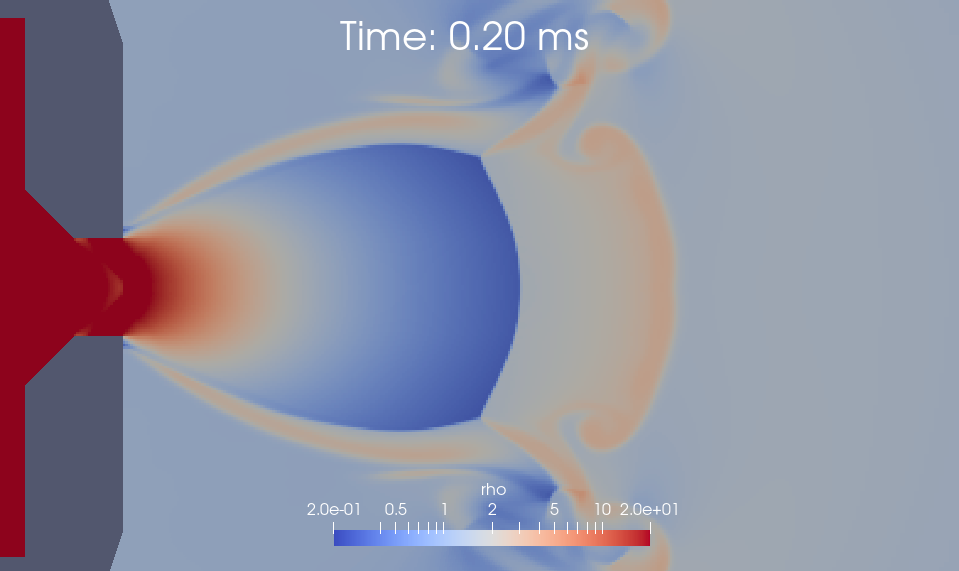
This example shows the transient exhaust of gas from a finite reservoir. The original experiment explored the jet as an analog of a volcanic eruption and provided images of the jet at various times.
Reference:
-
MM Orescanin, JM Austin and SW Kieffer (2010),
Unsteady high-pressure flow experiments with applications to explosive volcanic eruptions.
Journal of Geophysical Research 115 B06206. -
MM Orescanin and JM Austin (2010),
Exhaust of underexpanded jets from finite reservoirs.
Journal of Propulsion and Power 26(4): 744-753.
3.2. 2D/shear-layer-periodic

This two-dimensional flow has a positive x-velocity in the upper half of the domain and a negative x-velocity in the lower half. A finite-width shear layer with a linear variation in x-velocity separates these high-speed regions. The y-velocity is initially perturbed, most strongly in the middle of the domain, diminishing toward the north and south boundaries, which are ideal flat walls that allow slip. The west and east boundaries are connected such that the flow is periodic in the x-direction. The flow is allowed to evolve, with the initial shear layer vorticity rolling into distinct cores that are distorted as the acoustic waves propagate between the slip-wall boundaries. The animation above uses a grid-refinement factor of 4 and the corresponding simulation run time is a bit less than an hour on a workstation with a few cores. The input script checked into the repository has a lower factor of 2, which requires only a few minutes to run. Note that the animation shows three periods of the computed flow field: the original plus two copies translated in the x-direction.
4. Laminar flows of perfect gases
4.1. 2D/flat-plate-hakkinen-swbli
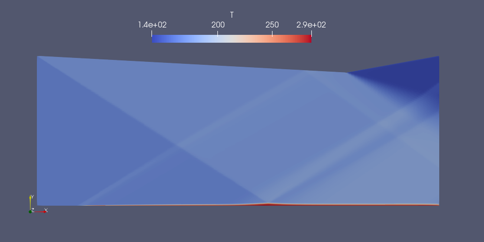
An oblique shock wave interacts with a laminar boundary layer on a flat flate. The boundary layer can be seen as the warmer temperture gas close to the lower boundary. The oblique shock generated at the leading edge of the upper boundary can be seen to arrive at the plate a little after half-way along the flow domain.
4.2. 2D/cylinder-type-iv-shock

The peak impingement pressure and heat-transfer to a cylinder can be amplified by more than an order of magnitude by having an oblique shock interact with the bow shock over the cylinder. This example models the flow discussed in Glass [1] and Moss et al. [2] and the experiment of Pot et al. [3]. The position of the oblique shock has been set to produce a Type IV pattern of interference, which results in the impingement of a hot jet on the cylinder surface at about 30 degrees below the horizontal axis.

References:
-
C. E. Glass (1999),
Numerical Simulation of Low-Density Shock-Wave Interactions,
NASA/TM-1999-209358. -
J. N. Moss, T. Pot, B. Chanetz and M. Lefebre (1999),
DSMC Simulation of Shock/Shock Interactions: Emphasis on Type IV Interactions,
https://ntrs.nasa.gov/citations/20040086965 -
T. Pot, B. Chanetz, M. Lefebre and P. Bouchardy (1999),
Fundamental Study of Shock/Shock Interference in Low Density Flow: Flowfield Measurements by DLCARS.,
Proceedings of the 21st International Symposium on Rarefied Gas Dynamics,
Marseille, 26-31 July 1998. Volume 2, pages 545-552.
5. Turbulent flows of perfect gases
5.1. 2D/flat-plate-turbulent-larc/nk-5.45Tw-sa
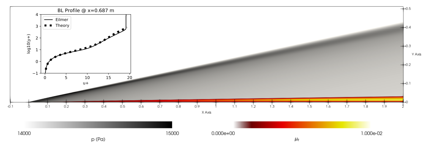
This example considers the solution of a high speed flow over a flat plate, using the Spalart-Allmaras one equation model to account for turbulence in the boundary layer. The grid and flow conditions are taken from NASA Langley’s Turbulence Modeling Resource website, specifically the 2DZPH high Mach number validation case, solved for a freestream Mach number of 5 and a ratio of wall temperature to freestream temperature of 5.450. 8500 iterations of the steady state solver were used to converge the solution, using a fine grid with 544x384 cells.
The black/grey colourmap shows pressure field, dominated by a viscous interaction shock formed at the start of the plate. Overlayed on the pressure is a red/orange colourmap of the turbulent viscosity \(\mu_t\), which is concentrated in the upper section of the boundary layer. The inset graph compares the solution to a Van Driest turbulent boundary layer profile computed at \(Re_\theta=10,000\), which corresponds to an x position of 0.687 meters from the start of the actual plate section. Good agreement is observed between the simulation and the theoretically predicted non-dimensional velocity \(u^+\).
6. Reacting gas flows
6.1. 2D/oblique-detonation-wave
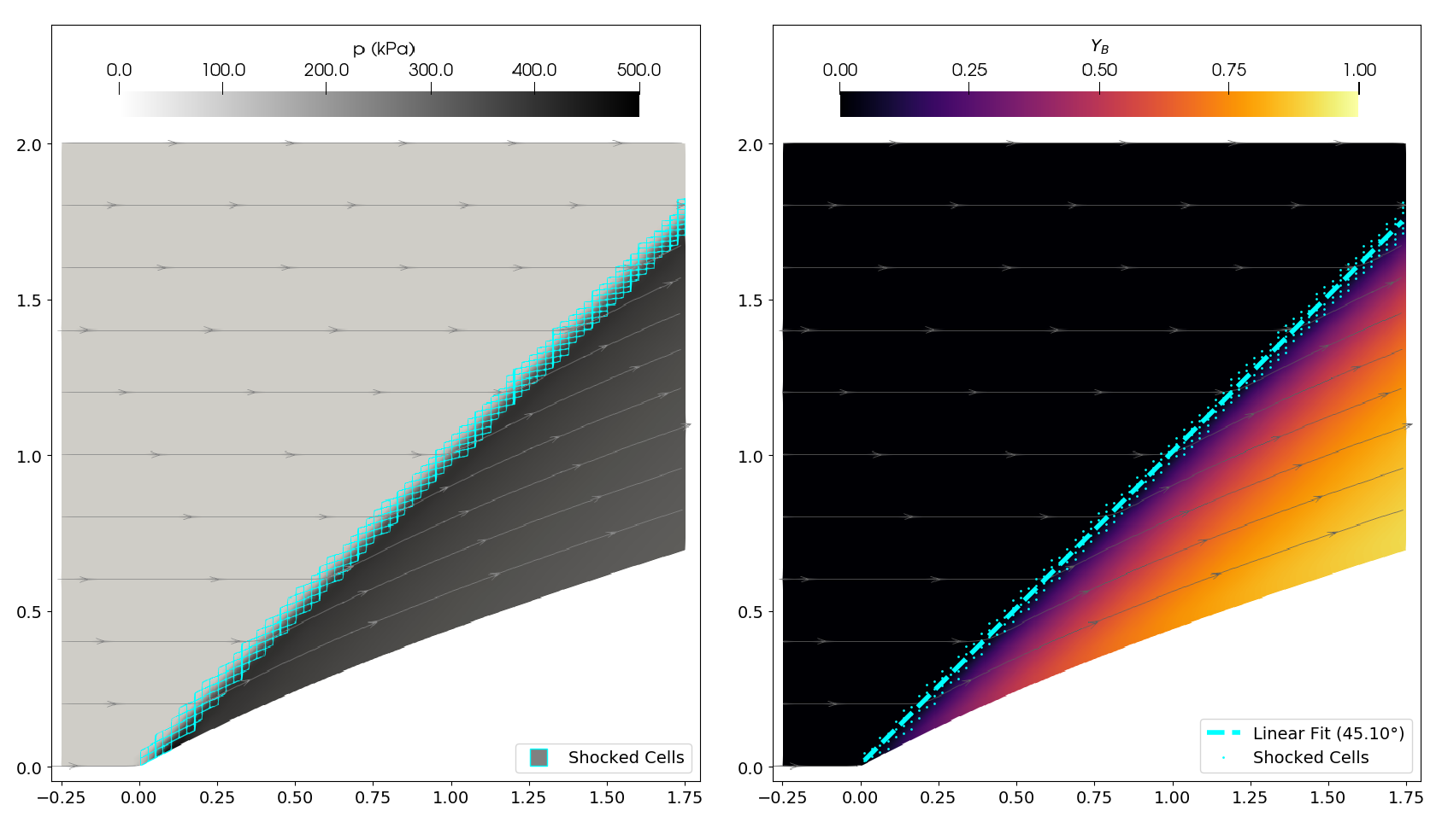
The flow in this example corresponds to an exact solution published by Powers and Aslam in 2006, in a paper calling for more widespread and rigorous verification of numerical codes used in aerospace research. The flow is inviscid and reacting, using a two-species single-step irreversible reaction which proceeds once a specified ignition temperature is reached. Here, the ignition temperaure is exceeded behing the shock. The curved ramp is designed in concert with the reaction rates to generate a straight detonation wave at \(45^\circ\), driven by an exothermic reaction that proceeds slowly as the flow travels further downstream.
The left hand image shows the pressure field, with the cells identified by the shock detector highlighted in light blue. The pressure is highest directly behind the shock and then falls as the reaction proceeds and the temperature increases. The procedure of this reaction is shown on the right; a colourmap of the product species mass fraction, along with a linear fit through the shock detected cells where the detonation wave is present. Though the example grid is not highly resolved, the angle of the linear fit and its explained variance are used in the internal integration tests to verify the reaction machinery and convection of multiple-species gases are interacting correctly with the rest of the code.
Reference:
-
Powers, J., and Aslam, T. (2006),
Exact Solution for Multidimensional Compressible Reactive Flow for Verifying Numerical Algorithms,
AIAA Journal, 44(2).
7. Flows with moving boundaries
7.1. 2D/moving-grid/piston-w-const-vel/simple

This example simulates the motion of a piston, at constant velocity, driving into ideal air. It is an example that shows the use of the moving grid capability in Eilmer. In the animation, you can see a fixed number of cells for the entire simulation. These cells move during the course of the simulation. In fact, it is is the user’s job to supply the grid motion in these types of simulation. This is done by specifying the velocities at the vertices in the grid.
The conditions for this simulation are:
-
piston speed: 293.5 m/s
-
initial pressure: 1.0e4 Pa
-
initial temperature: 278.8 K
With these conditions, the resulting shock speed is 554.35 m/s. This can be computed using the ideal shock relations. If these flow conditions look familiar, it is because they have been chosen to match conditions used in the classic Sod shock tube problem.
The conditions between the piston face and the shock have been computed analytically. They are:
-
pressure = 30.33 kPa
-
temperature = 397.9 K
7.2. 2D/moving-grid/rotating-square-simple

This example displays a square in Mach 6 free flight conditions, following a prescribed rotational motion. The implementation of dynamics builds on the ideas illustrated in the piston example above, and are defined by the user.
Taking \(\theta\) as the angle of the square face relative to incoming flow \((\theta_0 = 0)\), the dynamics were defined by the rotational velocity \(\omega\): \[\omega(t) = A \cos((2 \pi / t_f) \cdot t)\]
where \(A = 2000\) (rad/s). This formulation ensures a large sweep of angles are completed over the simulation time \([0,t_f]\), while also enusuring the square finishes at it’s starting angle relative to the incoming flow.
The inflow conditions for this simulation are:
-
freestream pressure: 760 Pa
-
freestream temperature: 71 K
-
freestream V: 1005.0 m/s
Results from the simulation are shown below (flow startup omitted):

Aerodynamic Forces
|

Aerodynamic Moment (about body centre)
|
8. High-temperature gas flows
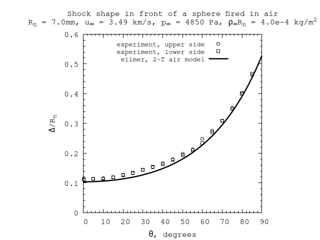
8.1. 2D/sphere-nonaka
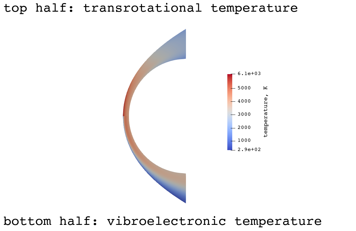
This example simulates the flow of air over a sphere. It is an example of using the two-temperature air model for high-speed flow. The particular conditions are chosen to replicate the physical experiments performed by Nonaka et al. (2000). Those conditions are Case 18 in Table 1. These conditions were chosen because they align with Figure 10 in their article. Figure 10 is one of the only cases where the full shock shape was reported. Having access to the full shock shape is very useful for validation. The conditions of this case are:
-
sphere radius : 7mm
-
free stream velocity : 3490 m/s
-
free stream pressure : 4850 Pa
-
free stream temperature : 293.0 K (assumed, not stated)
-
free stream composition : f_N2 = 0.767, f_O2 = 0.233
A comparison of the computed shock shape to the experiment is shown here.
Reference:
-
Nonaka, S., Mizuno, H., Takayama, K. and Park, C. (2000),
Measurement of Shock Standoff Distance for Sphere in Ballistic Range,
Journal of Thermophysics & Heat Transfer, 14(2).
8.2. 2D/wall-catalysis
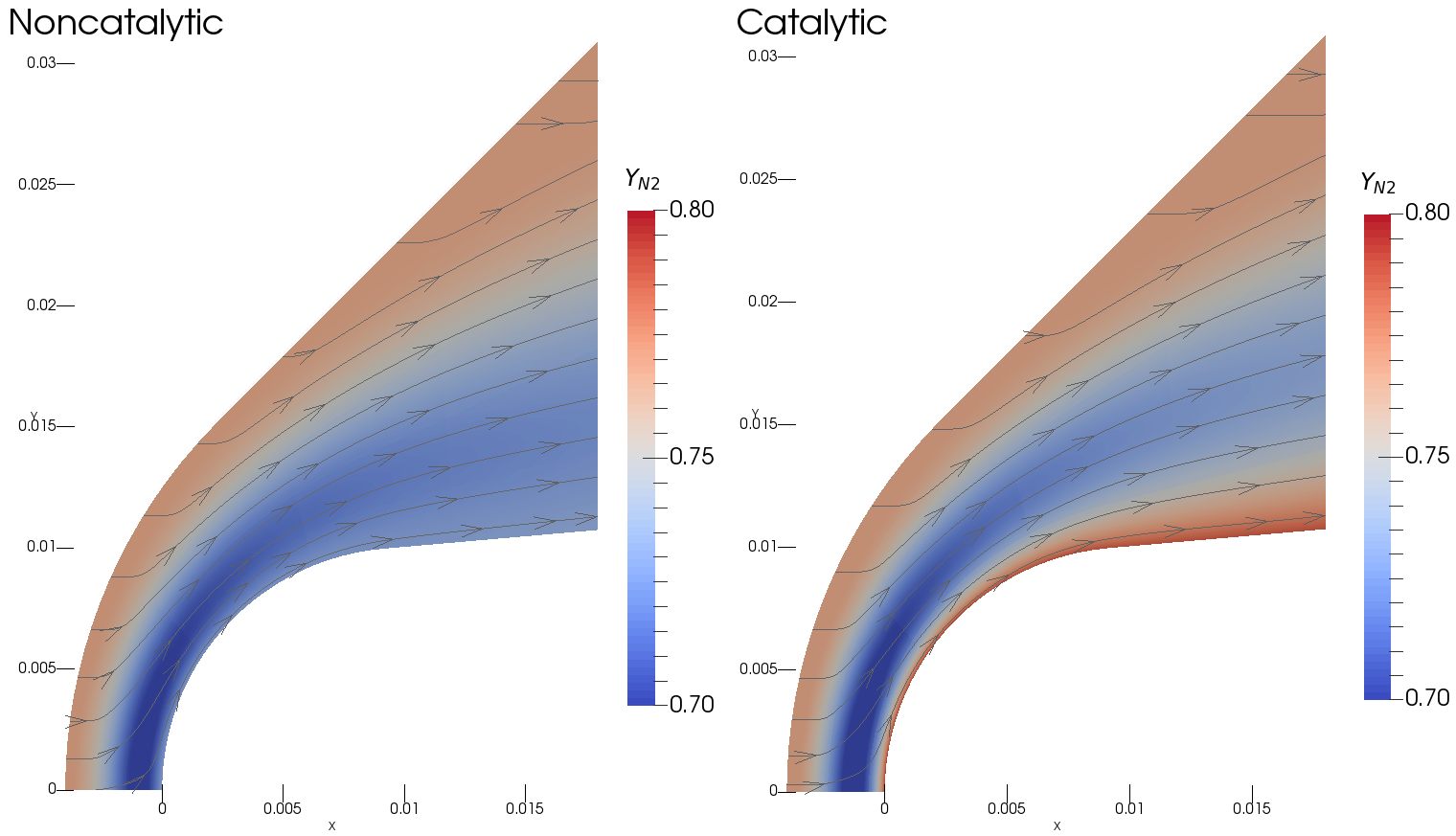
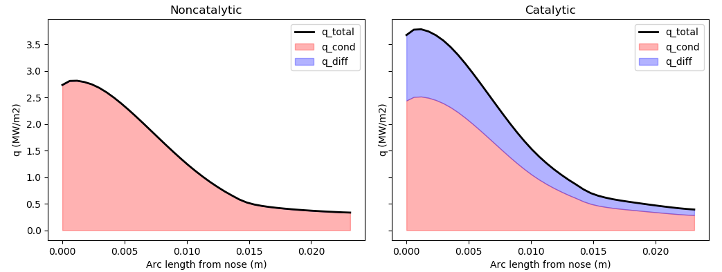
This example exercises the mass fraction boundary conditions for a blunt wedge with an elevated temperature of 2200K, immersed in a hypersonic flow at 6 km/s. The left hand image shows the mass fraction of molecular nitrogen (N2), using a normal fixed temperature wall where the mass fraction gradients are set to zero. Note the drop in N2 as the gas passes through the shock layer and begins to dissociate. In contrast the right hand image uses a fully catalytic wall, where the mass fraction values are set to their equilibrium composition --- effectively assuming that the wall accelerates the reaction rates all the way to completion. Note the layer of red against the wall of this image, demonstrating that the wall is forcing some of the nitrogen molecules to recombine, despite its elevated temperature.
This effect can significantly increase the heat transferred to the surface from the fluid, as shown in the figure below. The "q_diff" term represents the additional heat transfer from chemical activity at the surface, which is only present in the catalytic wall case.
9. Flows with Conjugate Heat Transfer (CHT)
9.1. 2D/cht-hollow-cylinder/transient-fluid-transient-solid

This example simulates the flow of air over a hollow cylinder and the induced heat transfer into the cylinder. It is an example of using the Conjugate Heat Transfer (CHT) solver in Eilmer for coupled fluid/solid domain simulations. In the CHT solver, the Navier-Stokes equations are solved on the fluid domain and an energy conservation equation is solved on the solid domain. A special boundary condition ensures the temperature and heat flux match at the interface between the solid and fluid domains. More details can be found in the article by Veeraragavan et al. (2016).
The particular conditions for this example are chosen to replicate the physical experiments performed by Wieting (1987). The simulation uses an explicit time integration scheme to simulate 5 seconds of flow. An animation of the solution above shows a bow shock quickly forming upstream of the cylinder before a slow but noticeable increase in the cylinder’s temperature can be observed. Wieting provides surface temperature measurements for this flow condition which can be used for validation purposes. A comparison of the surface temperature of the cylinder to the experiment is shown here.

Reference:
-
Veeraragavan, A., Beri, J. and Gollan, R. J. (2016),
Use of the Method of Manufactured Solutions for the Verification of Conjugate Heat Transfer Solvers,
Journal of Computational Physics, 307(308-320). -
Wieting, A. R. (1987),
Experimental Study of Shock Wave Interference Heating on a Cylindrical Leading Edge,
NASA Technical Memorandum, TM-100484.