T5 nozzle computation with specified throat-condition history
H. G. Hornung, 2023-07-26
The computation of the nozzle flow in T5 is normally performed with a block-marching scheme which takes much less time than a time-accurate method. However, if one wants to study the time-dependence of the flow in the test section, it is necessary to use the latter. For that case, it is most convenient to start from a known throat flow state, so that the whole of the flow is supersonic. Fortunately, it is a good approximation to compute the throat state with a one-dimensional equilibrium method in the usual way, from the initial shock-tube state, the shock speed and the reservoir pressure. Since the reservoir pressure varies with time in a known (measured) fashion, repeated applications of this method yield the flow state at the throat at discrete times. The software package Eilmer4 provides the feature of specifying an inflow boundary condition that depends on time, through a file that gives the flow state as a function of time. In this report I describe how this method is used to compute time traces of the nozzle exit conditions for two T5 runs.
1. Computation of the transient throat state
For this task I use the one-dimensional nozzle-flow code of the
gas-dynamics toolkit of the Centre for Hypersonics of the University
of Queensland which is called nenzf1d. The input to this code
consists of the initial shock tube state (gas composition, temperature
and pressure), the shock speed and the reservoir pressure, as
well as the specification of the equilibrium behavior of the gas
in the form of the files called gas.lua and
cea-air5species-gas-model.lua, and the relaxation behavior of the
gas in the form of the files called chem.lua and kinetics.lua.
In my case the gas is air and the model is the Bose/Candler
5-species 6-reaction 2-temperature model. In addition nenzf1d requires
the nozzle shape to be provided in the form of a few Bezier points.
In the case at hand the part of nenzf1d that computes the
one-dimensional flow through the nozzle is not needed, and only the
condition at the throat that it supplies is used. All the named
files as well as an example input file t5-air-2T.yaml and the
corresponding output file 47 accompany this report.
# Sample input file for nenzf1d is a YAML 1.1 file.
# t5-air-2T.yaml
# Data for T5 shot 2946
# HGH 2023-5-29
#
title: "T5-2916 2T-air with contoured nozzle."        # Any string will do.

species: ['N2', 'O2', 'N', 'O', 'NO']         # List
molef: {'N2': 0.79, 'O2': 0.21}               # Map of nonzero values will suffice.
# Gas model and reactions files need to be consistent with the species above.
# Gas model 1 is usually a CEAGas model file.
# Gas model 2 is a thermally-perfect gas model for the finite-rate chemistry.
gas-model-1: cea-air5species-gas-model.lua
gas-model-2: air-5sp-2T.lua
reactions: air-5sp-6r-2T.lua
reactions-file2: air-energy-exchange.lua

# Observed parameter values for shock-tube operation from Table 1 in Appendix A.
T1: 300         # K
p1: 45.0e3     # Pa
Vs: 4071.0      # m/s
pe: 47.0e6     # Pa
ar: 106.0       # contoured nozzle
# pp_ps: 0.0105   # From Figure 8.

meq_throat: 1.03  # To get supersonic condition with frozen-gas sound speed
C: 0.94           # estimate of Rayleigh_Pitot/(rho*V^2) for frozen gas at exit

# Define the expanding part of the nozzle as a schedule of diameters with position.
xi: [0.0000, 0.1, 0.2, 0.4, 0.6, 0.8, 1.0]
di: [0.030, 0.0625, 0.13,   0.21,   0.26,   0.290,   0.306]

# Optionally, we can adjust the stepping parameters for the supersonic expansion.
# x_end: 1.0
# t_final: 1.0e-3
# t_inc: 1.0e-10
# t_inc_factor: 1.0001
# t_inc_max: 1.0e-7
NENZF1D: 1D analysis of shock-tunnel with nonequilibrium nozzle flow. Revision-id: 61c8fa55 Revision-date: Mon Jun 27 20:46:03 2022 +1000 Compiler-name: ldc2 Build-date: Mon Aug 15 09:45:22 AM PDT 2022 T5-2916 2T-air with contoured nozzle. Initial gas in shock tube (state 1). pressure 45 kPa density 0.52048 kg/m^3 temperature 300 K H1 0.00187165 MJ/kg Incident-shock process to state 2. V2 439.594 m/s Vg 3631.41 m/s pressure 7739.5 kPa density 4.82007 kg/m^3 temperature 5040.27 K Reflected-shock process to state 5. Isentropic relaxation to state 5s. entropy 10095.8 J/kg/K H5s 15.8715 MJ/kg H5s-H1 15.8696 MJ/kg pressure 47000 kPa density 16.285 kg/m^3 temperature 8117.31 K Isentropic flow to throat to state 6 (Mach 1). V6 1774.71 m/s mflux6 17924.6 pressure 26538 kPa density 10.1 kg/m^3 temperature 7500.82 K Isentropic flow to slightly-expanded state 6e (Mach 1.03). V6e 1823.13 m/s mflux6e 17909.3 ar6e 1.00085 pressure 25670.5 kPa density 9.8234 kg/m^3 temperature 7465.81 K Isentropic expansion to nozzle exit of given area (state 7). area_ratio 106 V7 4913.36 m/s pressure 29.7586 kPa density 0.034416 kg/m^3 temperature 2910.7 K mflux7 17924.4 pitot7 814.62 kPa End of part A: shock-tube and frozen/eq nozzle analysis. Initializing gas state using CEA saved data Begin part B: continue supersonic expansion with finite-rate chemistry. Start position: x 3.93087e-05 m area-ratio 1.00085 Start condition: velocity 1859.98 m/s sound-speed 1858.13 m/s (v-V6e)/V6e 0.0202148 pressure 25670.5 kPa density 9.81517 kg/m^3 temperature 7465.81 K T_modes[0] 7465.81 K massf[N2] 0.683111 massf[O2] 0.00864601 massf[N] 0.048463 massf[O] 0.18372 massf[NO] 0.0760601 Exception thrown in nenzf1d.run! Exception message: Coefficients for CEA curve could not be determined. T=-nan
In the output file 47 the part of interest is the flow state
at the throat. This is given just after the line that states:
Begin part B: continue supersonic expansion with finite-rate chemistry.
This part of the output gives velocity, speed of sound, pressure,
temperature, vibrational temperature and composition. The first step
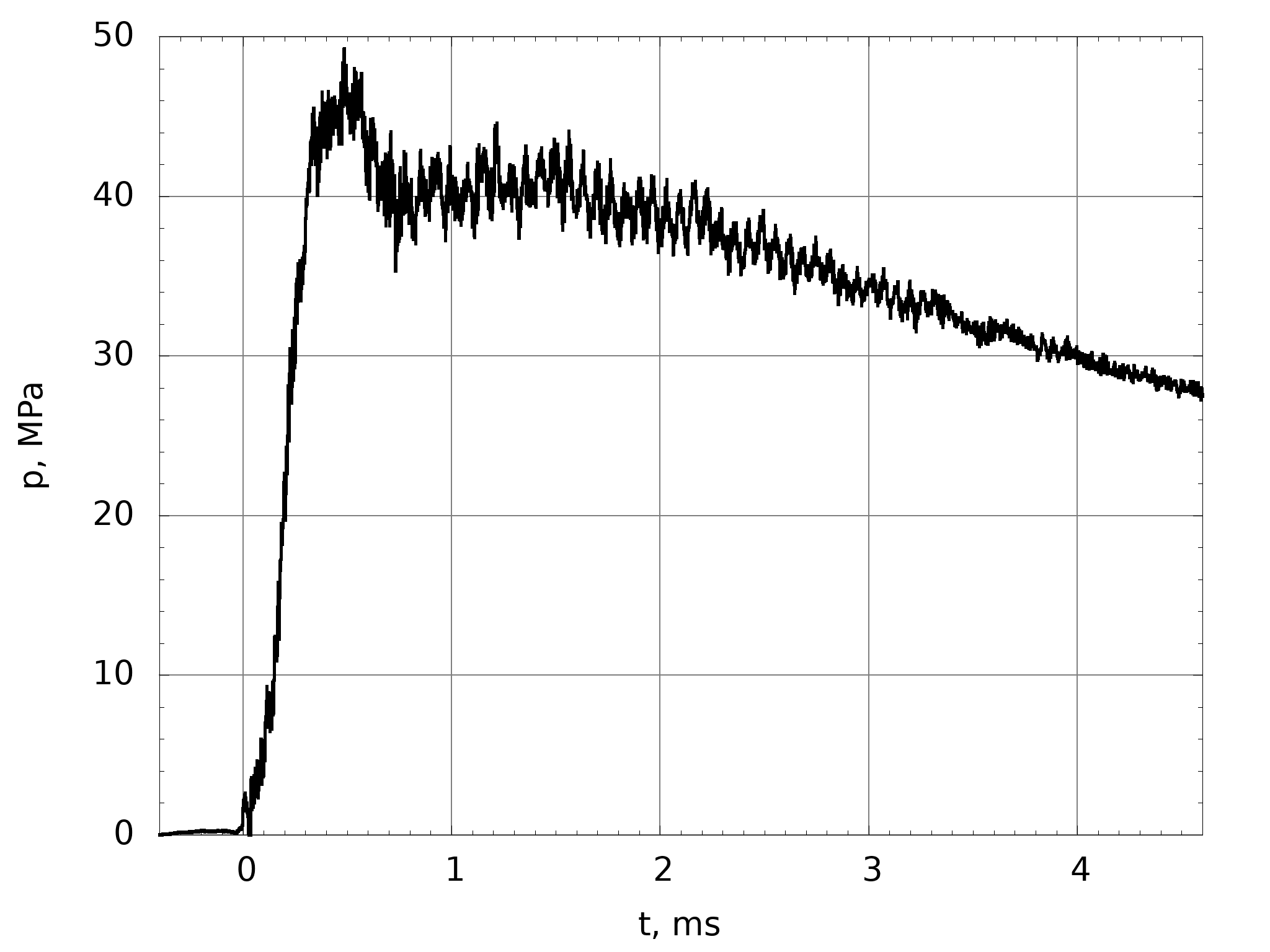
is to choose a point on the reservoir-pressure trace,
see figure 1, noting the time and the pressure. Then this
pressure is used in the input file to nenzf1d. The throat flow state
in the resulting output is then transcribed together with the time
into a line in the file "throat-file.dat" (an example of which
accompanies this report). This is repeated for other time/pressure
pairs with suitably densely
spaced times along the trace, till the period of interest is covered.
Since the boundary layer in the nozzle is partially turbulent, the
throat file needs an additional parameter for the turbulence model,
which in my case is the Spalart-Allmaras model.
2. Nozzle flow computation
The next step is to run the nozzle-start program in Eilmer4. (See
accompanying file t5ns.lua.) This requires as input the same gas
files, that are now actually used, as well as the nozzle profile
which is specified as a spline through many coordinate points.
In t5ns.lua the inflow
boundary condition is the file throat-file.dat which is invoked by
west=InFlowBC_Transient:new{fileName = "throat-file.dat"}
in the specification of the boundary conditions.
Running this computation with MPI and 48 processors takes about
one day with the resolution I have chosen (2560x92 cells),
heavily clustered towards the nozzle wall
for good resolution of the boundary layer.
With a partially turbulent boundary layer it is necessary to specify the transition point. Since the nozzle exit pressure is sensitive to the choice of the transition point, I chose the transition point by tuning it to give an exit pressure that matches the exit pressure measured at the mid point of the useful test time.
3. Results
The two conditions considered here were T5-2946 and T5-3029. Figure 2 shows the distribution of flow variables along the radius in the nozzle exit plane of T5-2946 at t=1.5ms. The best location of the transition point in this case was x=0.425m. The corresponding pressure traces are shown in figure 3.


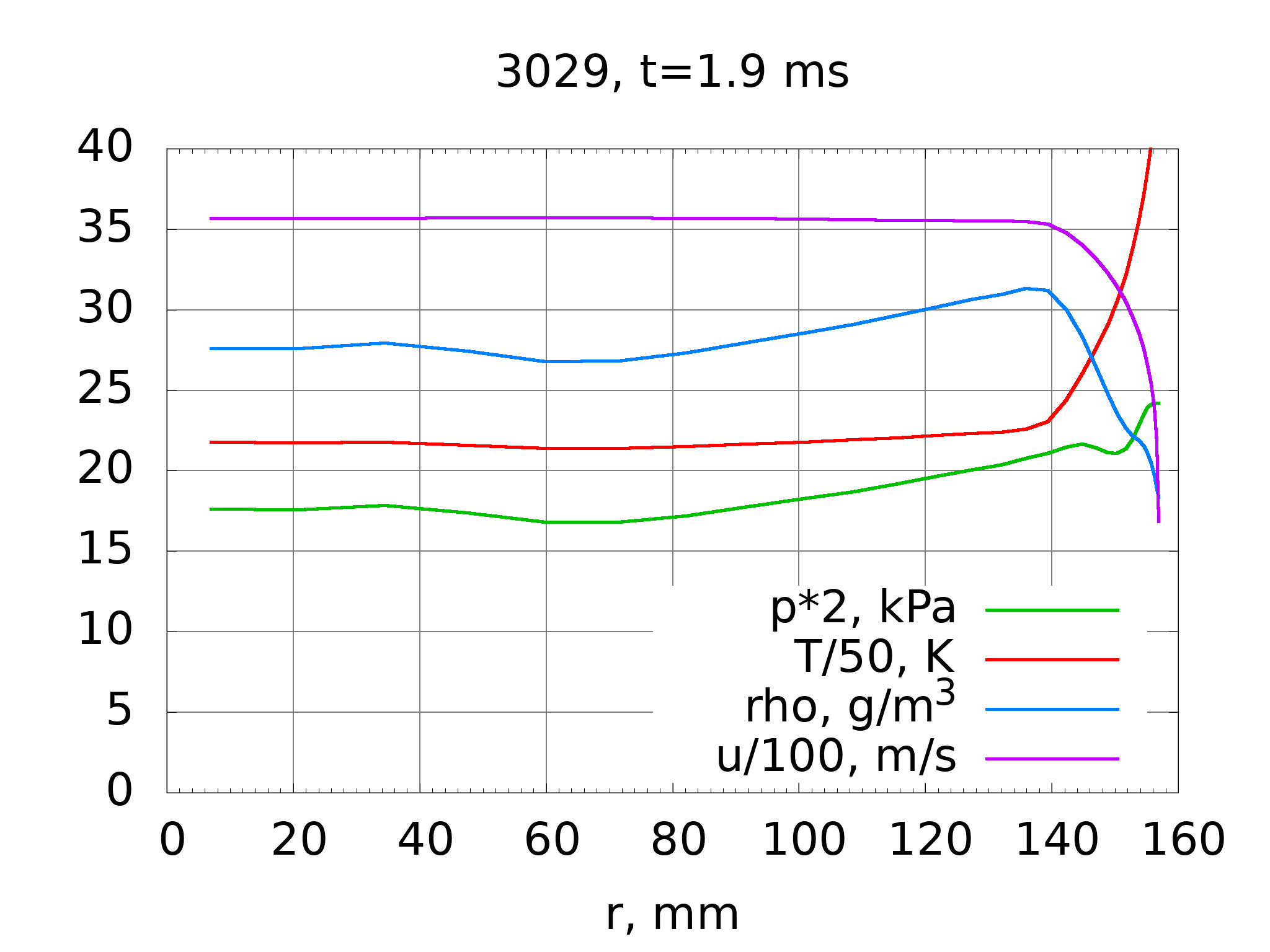
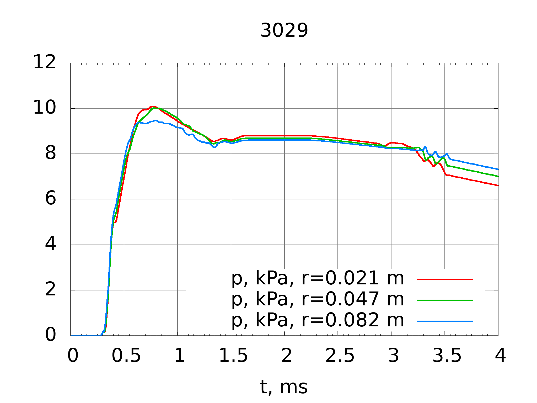
Figure 4 shows the distribution of flow variables along the radius in the nozzle exit plane of T5-3029 at t=1.9ms. The best location of the transition point in this case was x=0.4m.
4. Conclusions
A procedure is described by which it is possible to compute the time-dependent behavior of the test section conditions in T5. The procedure is applied to two particular T5 runs. All the files needed for this procedure accompany this report, in the hope that one of the graduate students can make the procedure less laborious and thus provide a useful tool for future use in T5 research.