Design Optimization of a Thrust Nozzle
Peter Jacobs, 2021-12-29
It is easy to include Eilmer flow simulations in an automatic optimization procedure. This note documents an example of determining the optimal shape of a classic, bell-shaped nozzle for a rocket motor.
1. Background
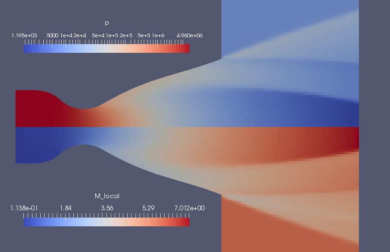
Rocket nozzles that are designed for producing maximum thrust have a bell-like profile1. An example flow field, displayed as pressure and Mach number images, is shown below in Figure 1. Gas enters the simulation domain at the left at subsonic, high-pressure and high-temperature conditions. This gas models the combustion products inside the rocket motor with a stagnation temperature of 3000 K and a stagnation pressure on 5 MPa. The gas accelerates toward the opening at the nozzle throat and, if we were to just let the gas vent to atmospheric conditions unbounded from this throat, we could achieve significant thrust. We can, however, obtain a higher thrust by adding a (divergent) supersonic part to the nozzle, as shown in the figure.
This example came from a 2017 class assignment in which students used the Eilmer CFD code to do their calculations. They were provided with an input script (shown later) that models a conical nozzle and a command script that runs a single flow simulation. They were then able to run test flows for particular nozzle shapes by editing a few parameters in the input script and then running the Eilmer code. Output from the flow simulation includes several snapshots of the entire flow field (that may be used to make pretty pictures, as shown above in Figure 1) and a small surface-loads file that contained enough data to compute the thrust on the expanding nozzle surface. The goal was to select values of the control parameters (that set the shape of the nozzle) so that they achieved maximum thrust in the axial direction.
2. Simulation of a particular nozzle
We start by setting up the simulation of the nozzle expansion flow path that is embedded in a more complete flow domain, including a bit of the subsonic flow upstream of the nozzle throat and some of the surrounds downstream of the nozzle exit. This allows the simulation to start with known stagnation conditions within the body of the motor and allows the transient flow to develop into a steady supersonic flow in the expanding part of the nozzle. Note that the expanding flow in figure 1 is not uniform and shows evidence of an oblique shock structure within the bell nozzle. Such detail is handled implicitly within the simulation and all we need to inspect in detail is the pressure distribution along the expanding wall. This is provided in a "loads" file writen by Eilmer.
2.1. Defining the nozzle flow path
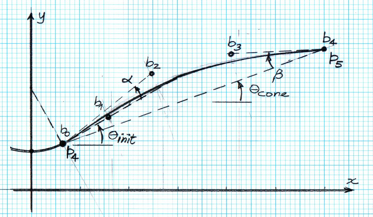
The supersonic expansion part of the bell nozzle is set up as a variation of a straight conical nozzle.
Four parameters define the particular shape of the bell nozzle via the control points
of a Bezier curve.
These parameters are set at about a third of the way into the script and are the angles: theta_cone, theta_init, alpha and beta.
The profile of the divergent part of the nozzle consists of a circular arc,
followed by a Bezier curve.
The Bezier curve has 5 points: b0, b1, b2, b3 and b4.
The angle theta_init is also the angle of the polygon segment b0-b1,
so that we get continuity of slope with the arc from the nozzle throat.
The angle alpha sets the position of point b2, relative to the start (b0).
This allows us to expand even further than the arc or start to compress the flow.
We have a choice.
The angle theta_cone sets the position of exit point b4 and so,
in combination with the initial angle, determines the diameter of the nozzle exit.
The nozzle length (in the x-direction) remains fixed.
The other control angle, beta, sets the position of b3 relative to b4,
so that we can choose the exit angle of the flow at the nozzle wall.
With theta_cone equal to theta_init and alpha and beta both set to zero, we have a straight
conical nozzle.
2.2. Input script
-- nozzle.lua
-- Optimize an axisymmetric bell nozzle for ENGG7601 assignment.
-- Peter J. 2017-09-06 adpated from the Back nozzle simulation,
-- hence the dimensions in inches.
--
config.title = "Flow through a rocket nozzle."
print(config.title)
nsp, nmodes = setGasModel('ideal-air-gas-model.lua')

-- The stagnation gas represents a reservoir condition inside the rocket motor.
-- The low_pressure_gas is an arbitrary fill condition for two of the blocks.
-- It will be swept away.
-- The external_stream will provide an environment for the rocket's exhaust gas.
stagnation_gas = FlowState:new{p=5.0e6, T=3000.0}
low_pressure_gas = FlowState:new{p=30.0, T=300.0}
external_stream = FlowState:new{p=8.0e3, T=300.0, velx=2.0e3}

-- Define geometry of our rocket motor and nozzle.
-- The original paper by Back etal (for a lab experiment on supersonic nozzles)
-- specifies sizes in inches, Eilmer works in metres.
inch = 0.0254 -- metres
L_subsonic = 3.0 * inch
L_nozzle = 6.0 * inch
R_tube = 1.5955 * inch
R_throat = 0.775 * inch
R_curve = 1.55 * inch -- radius of curvature of throat profile
--
-- The following three angles set the shape of the supersonic expansion
-- part of the nozzle.
-- The profile is defined by a circular arc, followed by a Bezier-curve
-- with 5 defining points {b0, b1, b2, b3, b4} whose positions are set
-- by the angles theta_init, alpha, beta, theta_cone.
-- With theta_init=theta_cone defining the nominally-straight conical nozzle.
-- You may vary alpha and beta away from zero, to generate a curve
-- to replace the straight profile of the nominal cone.
-- The values alpha=0 and beta=0 will give you a Bezier curve that
-- happens to be a straight line.
-- Set theta_init > theta_cone to get a rapidly expanding thrust surface.
--
theta_cone = math.rad(30.0) -- nominal straight-cone angle
theta_init = math.rad(30.0) -- starting angle for thrust nozzle
alpha = math.rad(0.0)  -- angle for setting b2 in Bezier curve
beta = math.rad(0.0)  -- angle for setting b3 in Bezier curve

-- Compute the centres of curvature for the contraction profile.
height = R_throat + R_curve
hypot = R_tube + R_curve
base = math.sqrt(hypot*hypot - height*height)
centre_A = Vector3:new{x=0.0, y=height}
centre_B = Vector3:new{x=-base, y=0.0}
fraction = R_tube/hypot
intersect_point = centre_B + Vector3:new{x=fraction*base, y=fraction*height}

-- Assemble nodes from coordinates.
z0 = Vector3:new{x=-L_subsonic, y=0.0}
p0 = Vector3:new{x=-L_subsonic, y=R_tube}
z1 = Vector3:new{centre_B} -- initialize from a previously defined Node
p1 = centre_B + Vector3:new{x=0.0, y=R_tube}
p2 = Vector3:new{intersect_point}
z2 = Vector3:new{x=p2.x, y=0.0}  -- on the axis, below p2
z3 = Vector3:new{x=0.0, y=0.0}
p3 = Vector3:new{x=0.0, y=R_throat}
-- Compute the details of the conical nozzle.
-- Circular arc to p4, followed by straight line at angle theta to p5.
p4 = Vector3:new{x=R_curve*math.sin(theta_init),
		 y=height-R_curve*math.cos(theta_init)}
z4 = Vector3:new{x=p4.x, y=0.0}
L_cone = L_nozzle - p4.x
R_exit = p4.y + L_cone*math.tan(theta_cone)
p5 = Vector3:new{x=p4.x+L_cone, y=R_exit}
z5 = Vector3:new{x=p5.x, y=0.0}
-- Final nodes define the Bezier curve.
b0 = p4
b1 = p4 + 0.2*L_cone*Vector3:new{x=1.0, y=math.tan(theta_init)}
b2 = p4 + 0.4*L_cone*Vector3:new{x=1.0, y=math.tan(theta_init+alpha)}
b3 = p5 - 0.3*L_cone*Vector3:new{x=1.0, y=math.tan(theta_cone-beta)}
b4 = p5
-- Some space downstream of the nozzle exit
z6 = Vector3:new{x=z5.x+L_nozzle, y=0.0}
p6 = Vector3:new{x=z6.x, y=R_exit}
q5 = Vector3:new{x=z5.x, y=2*R_exit}
q6 = Vector3:new{x=z6.x, y=q5.y}

north0 = Polyline:new{segments={Line:new{p0=p0,p1=p1},
				Arc:new{p0=p1,p1=p2,centre=centre_B},
				Arc:new{p0=p2,p1=p3,centre=centre_A}}}
east0west1 = Line:new{p0=z3, p1=p3}
south0 = Line:new{p0=z0, p1=z3}
west0 = Line:new{p0=z0, p1=p0}
north1 = Polyline:new{segments={Arc:new{p0=p3,p1=p4,centre=centre_A},
				Bezier:new{points={b0, b1, b2, b3, b4}}}}
east1 = Line:new{p0=z5, p1=p5}
south1 = Line:new{p0=z3, p1=z5}
-- The subsonic and supersonic parts of the nozzle have complicated edges.
patch0 = CoonsPatch:new{north=north0, east=east0west1, south=south0, west=west0}
patch1 = CoonsPatch:new{north=north1, east=east1, south=south1, west=east0west1}
-- The downstream region is just two rectangular boxes.
patch2 = CoonsPatch:new{p00=z5, p10=z6, p11=p6, p01=p5}
patch3 = CoonsPatch:new{p00=p5, p10=p6, p11=q6, p01=q5}

-- Define the blocks, boundary conditions and
-- set the discretisation to join cells consistently.
nx0 = 50; nx1 = 100; nx2 = 80; ny = 30
grid0 = StructuredGrid:new{psurface=patch0, niv=nx0+1, njv=ny+1}
grid1 = StructuredGrid:new{psurface=patch1, niv=nx1+1, njv=ny+1}
grid2 = StructuredGrid:new{psurface=patch2, niv=nx2+1, njv=ny+1}
grid3 = StructuredGrid:new{psurface=patch3, niv=nx2+1, njv=ny+1}
subsonic_region = FluidBlock:new{grid=grid0, initialState=stagnation_gas}
supersonic_region = FluidBlock:new{grid=grid1, initialState=low_pressure_gas}
downstream_region = FluidBlock:new{grid=grid2, initialState=low_pressure_gas}
external_region = FluidBlock:new{grid=grid3, initialState=external_stream}

-- History locations near throat and exit
setHistoryPoint{ib=1, i=1, j=1}
setHistoryPoint{ib=1, i=nx1-1, j=1}

-- Boundary conditions for all of the blocks.
-- First stitch together adjoining blocks,
identifyBlockConnections()
-- then, directly specify the stagnation conditions for the subsonic inflow.
subsonic_region.bcList['west'] = InFlowBC_FromStagnation:new{stagnationState=stagnation_gas}
-- to get loads on thrust surface, add that boundary condition to the group
supersonic_region.bcList['north'] = WallBC_WithSlip:new{group="loads"}
downstream_region.bcList['east'] = OutFlowBC_Simple:new{}
external_region.bcList['east'] = OutFlowBC_Simple:new{}
external_region.bcList['west'] = InFlowBC_Supersonic:new{flowState=external_stream}

-- Do a little more setting of global data.
config.axisymmetric = true
config.flux_calculator = "adaptive"
config.max_time = 1.0e-3  -- seconds
config.max_step = 50000
config.dt_init = 1.0e-7
config.dt_plot = 0.1e-3
config.dt_history = 10.0e-6
config.dt_loads = 1.0e-3
config.write_loads = true
2.3. Running a simulation
With a gas model input file containing
model = "IdealGas"
species = {'air'}
we can now run a simulation with the commands
prep-gas ideal-air.inp ideal-air-gas-model.lua
e4shared --prep --job=nozzle
e4shared --run --job=nozzle --verbosity=1
e4shared --post --job=nozzle --tindx-plot=all --vtk-xml --add-vars="mach,pitot,total-p,total-h"
This particular simulation takes about 86 seconds to run 3740 steps on a Lenovo ThinkPad laptop with an Intel Core i7-8665U processor. While running, the htop command indicates that the calculation was getting about 330% of CPU. This is fair for a shared-memory multi-block simulation that is not well load-balanced.
The post-processing command was used to get some Paraview plotting files for viewing and is not necessary for estimating the thrust performance of the nozzle expansion as 1954 Newtons. That information comes from the "loads" file for the surface in the supersonic part of the nozzle.
2.4. The loads file
At the end of the simulation, there will be a loads directory and within that one or more
time-snapshot directories containing the actual loads files.
The first four lines of the loads file are:
# t = 0.00100001
# 1:pos.x 2:pos.y 3:pos.z 4:n.x 5:n.y 6:n.z 7:area 8:cellWidthNormalToSurface 9:outsign 10:p 11:rho 12:T 13:velx 14:vely 15:velz 16:mu 17:a 18:Re 19:y+ 20:tau_wall_x 21:tau_wall_y 22:tau_wall_z 23:q_total 24:q_cond 25:q_diff
8.6901831091239028e-04 1.9704191291093600e-02 0.0000000000000000e+00 -2.2078491087414227e-02 9.9975624040628175e-01 0.0000000000000000e+00 3.4254956041529100e-05 6.5681606367797105e-04 1 2.1826407390037715e+06 3.2098242206973855e+00 2.3684428227672779e+03 1.1268801560101706e+03 2.4885879652968022e+01 0.0000000000000000e+00 1.8469051721849357e-05 9.7569599305231236e+02 0.0000000000000000e+00 0.0000000000000000e+00 0.0000000000000000e+00 0.0000000000000000e+00 0.0000000000000000e+00 0.0000000000000000e+00 0.0000000000000000e+00 0.0000000000000000e+00
2.6053604868778481e-03 1.9780919035538712e-02 0.0000000000000000e+00 -6.6192423757590338e-02 9.9780687662347545e-01 0.0000000000000000e+00 3.4388344185924577e-05 6.5944989617703676e-04 1 1.9544084590699985e+06 2.9655698392620535e+00 2.2954565422634796e+03 1.1878342892646756e+03 7.8798445341315372e+01 0.0000000000000000e+00 1.8469051721849357e-05 9.6054475877413745e+02 0.0000000000000000e+00 0.0000000000000000e+00 0.0000000000000000e+00 0.0000000000000000e+00 0.0000000000000000e+00 0.0000000000000000e+00 0.0000000000000000e+00 0.0000000000000000e+00
For each line of data, we need to pick up the values for unit normal in the x-direction 4:n.x,
the cell-face area 7:area, and the pressure 10:p.
Note that, in an axisymmetric simulation such as this one, the area of the face is per radian
around the axis of symmetry.
3. Turning the input script into a template
So far, we have set up to manually run a single flow analysis simulation but, when running simulations within an automatic optimization process, we want to be able to generate Eilmer input scripts with specific values of the shape parameters. To do this, we turn the input script above into a "template" that has target strings instead of specific numbers. We change just four lines.
theta_cone = math.rad($theta_cone) -- nominal straight-cone angle
theta_init = math.rad($theta_init) -- starting angle for thrust nozzle
alpha = math.rad($alpha)  -- angle for setting b2 in Bezier curve
beta = math.rad($beta)  -- angle for setting b3 in Bezier curve
4. The optimization program
The following Python program codifies our process of setting up and running specific simulations based on out template input script.
The core of the program is the objective function that takes a list of parameter values,
sets up and runs a simulation, and returnss the simulated thrust on the expanding nozzle wall.
Note that we have used a thread-safe queue to get a unique job identity for each call
to the objective function.
This allows us to run more than one instance of the objective function concurrently,
which is handy because our implementation of the Nelder-Mead minimizer can replace more than
one simplex point with each step4.
The main function, toward the end of the code, can be run in one of several ways.
It can run just a single simulation, or evaluate a single call to the objective function,
or let the Nelder-Mead minimizer do its thing, running many simulations.
#! /usr/bin/env python3
# optimize.py
# Automate the running of the flow simulations while searching
# for the optimum parameters (angles) that define the nozzle shape.
#
# To monitor the progress of the optimizer, you can run the command:
# tail -f progress.txt
# to see the result of each objective evaluation.
#
# PJ, 2018-03-04, take bits from nenzfr
#     2021-12-22, update to accommodate loads-file changes, use nelmin
#                 and run jobs in their own directories

import sys, os
DGDINST = os.path.expandvars("$HOME/dgdinst")
sys.path.append(DGDINST)

import shutil, shlex, subprocess, queue
import string, math
import time
from gdtk.numeric.nelmin import minimize, NelderMeadMinimizer

start_time = time.time()
progress_file = open("progress.txt", 'w')
progress_file.write("# job wall_clock params[0] params[1] params[2] params[3] thrustx\n")
progress_file.flush()
# Each of the Eilmer simulations will be run in its own directory, identified by job number,
# so that it can be run independently of all other simulations.
# We will use a queue to regulate the specification of this job number.
obj_eval_queue = queue.Queue()
obj_eval_queue.put(0)

def run_command(cmdText, jobDir, logFile=None):
    """
    Run the command as a subprocess in directory jobDir.
    If a logFile name is provided, capture stdout+stderr and write to that file,
    else just let those streams go to the console.
    """
    # Flush before using subprocess to ensure output
    # text is in the right order.
    sys.stdout.flush()
    if (type(cmdText) is list):
        args = cmdText
    else:
        args = shlex.split(cmdText)
    # print("jobDir:", jobDir, "cmdText:", " ".join(args)) # debug
    captureFlag = True if logFile else False
    result = subprocess.run(args, cwd=jobDir, check=True, capture_output=captureFlag)
    if captureFlag:
        f = open(logFile, 'w')
        f.write(result.stdout.decode())
        f.write(result.stderr.decode())
        f.close()
    return result.returncode

def prepare_input_script(substituteDict, jobDir):
    """
    Prepare the actual input file for Eilmer4 from a template
    which has most of the Lua input script in place and just
    a few place-holders that need to be substituted for actual
    values.
    """
    fp = open("nozzle.template.lua", 'r')
    text = fp.read()
    fp.close()
    template = string.Template(text)
    text = template.substitute(substituteDict)
    fp = open(jobDir+"/nozzle.lua", 'w')
    fp.write(text)
    fp.close()
    return

def run_simulation(param_dict, jobDir):
    """
    Prepare and run a simulation in it own directory.
    We do this so that several simulations may run concurrently
    and so that we can easily find the data files later.
    """
    if not os.path.exists(jobDir): os.mkdir(jobDir)
    shutil.copy('ideal-air.inp', jobDir)
    logFile = jobDir+'.log'
    run_command('prep-gas ideal-air.inp ideal-air-gas-model.lua', jobDir, logFile)
    prepare_input_script(param_dict, jobDir)
    run_command('e4shared --prep --job=nozzle', jobDir, logFile)
    run_command('e4shared --run --job=nozzle --max-cpus=4 --verbosity=1', jobDir, logFile)
    return

def post_simulation_files(jobDir):
    """
    Postprocess a simulation is its own directory.
    Although not used by the optimizer, this function may be handy
    when exploring the behaviour of the optimization procedure.
    """
    run_command('e4shared --post --job=nozzle --tindx-plot=all'+
                ' --vtk-xml --add-vars="mach,pitot,total-p,total-h"', jobDir)
    run_command('e4shared --post --job=nozzle --slice-list="1,0,:,0"'+
                ' --output-file="nozzle-throat.data"', jobDir)
    run_command('e4shared --post --job=nozzle --slice-list="1,$,:,0"'+
                ' --output-file="nozzle-exit.data"', jobDir)
    return

def neg_thrust(tindx, jobDir):
    """
    Read the loads file and return the x-component of thrust.

    Input:
    tindx : integer specifying which loads file to inspect
    jobDir : the dedicated directory for the simulation files.
    """
    fileName = jobDir+'/loads/t%04d/b0001.t%04d.loads.dat' % (tindx, tindx)
    print("Estimating thrust from loads file ", fileName) # debug
    f = open(fileName, 'r')
    thrustx = 0.0
    for line in f.readlines():
        items = line.strip().split()
        if items[0] == '#': continue
        if len(items) < 10: break
        dA = float(items[6]) # 7:area per radian for axisymmetric simulation
        nx = float(items[3]) # 4:n.x
        p = float(items[9]) # 10:p
        thrustx = thrustx + 2*math.pi*dA*nx*p
    print("thrustx=", thrustx) # debug
    return thrustx

def objective(params, *args):
    """
    Given a list of parameter values, run a simulation and compute the thrust.
    Since the thrust is in the negative x-direction, large negative values are good.
    The minimizer will drive toward good values.
    """
    global start_time # Immutable.
    global progress_file # Shared output stream, hopefully not too messed up.
    global obj_eval_queue # Thread-safe.
    job_number = obj_eval_queue.get()
    job_number += 1
    obj_eval_queue.put(job_number)
    print("Start job number:", job_number)
    pdict = {"theta_init":params[0], "alpha":params[1],
             "beta":params[2], "theta_cone":params[3]}
    jobDir = 'job-%04d' % job_number
    run_simulation(pdict, jobDir)
    # Note that, if we run an Eilmer simulation several times,
    # there may be several loads files, indexed in order of creation.
    # We want the most recent, if we are in the optimization process.
    f = open(jobDir+'/loads/nozzle-loads.times', 'r')
    tindx = 0
    for line in f.readlines():
        items = line.strip().split()
        if items[0] == '#': continue
        if len(items) < 2: break
        tindx = int(items[0])
    thrustx = neg_thrust(tindx, jobDir)
    progress_file.write("%d %.1f %.4f %.4f %.4f %.4f %.2f\n" %
                        (job_number, time.time()-start_time, params[0],
                         params[1], params[2], params[3], thrustx))
    progress_file.flush() # so that we can see the results as simulations run
    return thrustx

def main():
    """
    This script was built in stages.
    The if-statements are for testing the functions as the script
    was being developed. They might be still useful for exploring.
    """
    if 0:
        print("Let's run a simulation.")
        pdict = {"theta_init":30.0, "alpha":0.0, "beta":0.0, "theta_cone":30.0}
        run_simulation(pdict, "job-0000")
    if 0:
        print("Compute thrust from previously run simulation.")
        print("thrust=", neg_thrust(0, 'job-0000'))
    if 0:
        print("Evaluate objective function.")
        params = [30.0, 0.0, 0.0, 30.0] # [theta_init, alpha, beta, theta_cone]
        obj_eval_number = 1
        objv = objective(params)
        print("objective value=", objv)
    if 1:
        print("Let the optimizer take control and run the numerical experiment.")
        x0 = [30.0, 0.0, 0.0, 30.0] # [theta_init, alpha, beta, theta_cone] degrees
        result = minimize(objective, x0, [2.0, 2.0, 2.0, 2.0],
                          options={'tol':1.0e-4, 'P':2, 'maxfe':60, 'n_workers':2})
        print('optimized result:')
        print('  x=', result.x)
        print('  fx=', result.fun)
        print('  convergence-flag=', result.success)
        print('  number-of-fn-evaluations=', result.nfe)
        print('  number-of-restarts=', result.nrestarts)
        print('  vertices=', [str(v) for v in result.vertices])
    #
    print("overall calculation time:", time.time()-start_time)
    return

# Let's actually do some work...
main()
progress_file.close()
5. Results
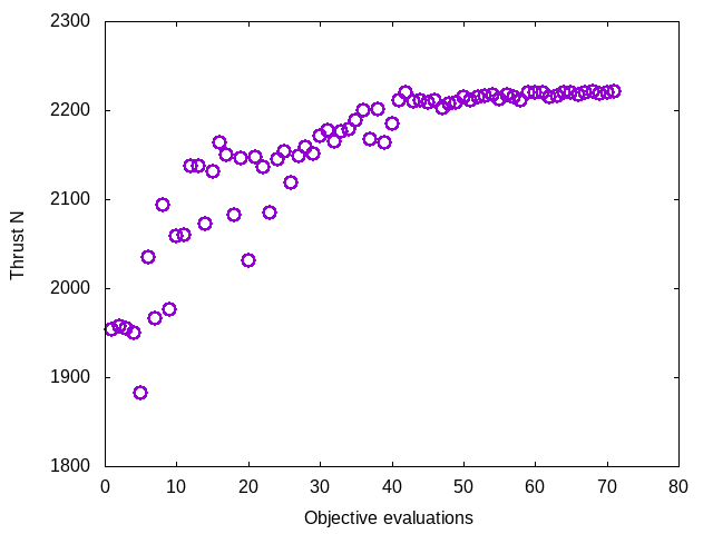
Replacing two simplex points per step and running the objective function evaluations with two workers in the tead-pool, the tail-end of the console output is:
optimized result:
  x= [29.678627533594543, -6.232721263775233, 5.956211556232702, 18.49358284183389]
  fx= -2220.791439092127
  convergence-flag= False
  number-of-fn-evaluations= 71
  number-of-restarts= 0
  vertices= ['Vertex(x=[29.67862753 -6.23272126  5.95621156 18.49358284], f=-2220.791439092127)', 'Vertex(x=[29.27443431 -6.21183191  5.78719484 18.03676979], f=-2220.769113094416)', 'Vertex(x=[29.28534293 -6.17598784  6.12646338 17.88696286], f=-2220.4961864985025)', 'Vertex(x=[29.4983822  -6.31313774  6.90884094 18.14101969], f=-2220.414532010557)', 'Vertex(x=[29.48168364 -5.51494113  5.86079823 18.19524534], f=-2220.3968307587793)']
overall calculation time: 4692.7158970832825
It shows that the overall run time is significantly less than one might expect for 71 simulations at 85 seconds each (6035 seconds). Thus it seems that we have made good use of all 8 hyperthreads on the Thinkpad’s processor.
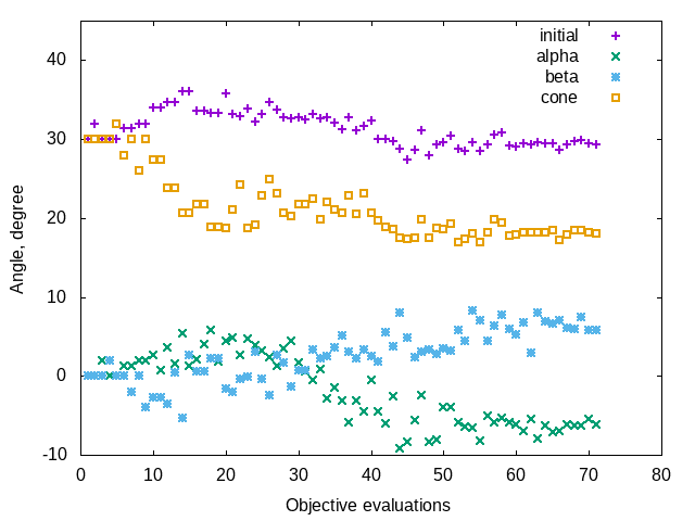
The progress.txt file that is used to accumulate values of parameters and the objective
during the optimization process is good for showing the history of the calculations.
As shown below, in Figure 3, the optimizer makes an improvement of about 13% on the thrust applied to
the supersonic part of the nozzle expansion.
References
-
[1] Rao, G. V. R. (1958). Exhaust nozzle contour for optimum thrust. Jet Propulsion, vol 28(5), pp 377—382.
-
[2] J.A. Nelder and R. Mead (1965) A simplex method for function minimization. Computer Journal, Volume 7, pp 308-313.
-
[3] R. O’Neill (1971) Algorithm AS47. Function minimization using a simplex algorithm. Applied Statistics, Volume 20, pp 338-345.
-
[4] Donghoon Lee and Matthew Wiswall (2007) A parallel implementation of the simplec function minimization routine. Computational Economics Volume 30, pp 171-187.